Note
Go to the end to download the full example code
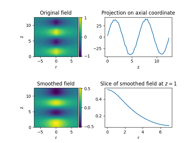
2.22 Visualizing a scalar field
This example displays methods for visualizing scalar fields.
import matplotlib.pyplot as plt
import numpy as np

from pde import CylindricalSymGrid, ScalarField

# create a scalar field with some noise
grid = CylindricalSymGrid(7, [0, 4 * np.pi], 64)
data = ScalarField.from_expression(grid, "sin(z) * exp(-r / 3)")
data += 0.05 * ScalarField.random_normal(grid)

# manipulate the field
smoothed = data.smooth()  # Gaussian smoothing to get rid of the noise
projected = data.project("r")  # integrate along the radial direction
sliced = smoothed.slice({"z": 1})  # slice the smoothed data

# create four plots of the field and the modifications
fig, axes = plt.subplots(nrows=2, ncols=2)
data.plot(ax=axes[0, 0], title="Original field")
smoothed.plot(ax=axes[1, 0], title="Smoothed field")
projected.plot(ax=axes[0, 1], title="Projection on axial coordinate")
sliced.plot(ax=axes[1, 1], title="Slice of smoothed field at $z=1$")
plt.subplots_adjust(hspace=0.8)
plt.show()
Total running time of the script: (0 minutes 0.316 seconds)