4.3.1 pde.grids.boundaries package
This package contains classes for handling the boundary conditions of fields.
4.3.1.1 Boundary conditions
The mathematical details of boundary conditions for partial differential equations are
treated in more detail in the
documentation document.
Since the pde package only supports orthogonal grids, boundary conditions
generally need to be applied at both ends of each axis.
Consequently, methods expecting boundary conditions typically receive a dictionary of
conditions for each axes:
field = pde.fields.scalar.ScalarField(UnitGrid([16, 16], periodic=[True, False]))
field.laplace(bc={"x": bc_x, "y-": bc_y_lower, "y+": bc_y_upper})
If both sides of an axis have the same boundary condition, they can be specified
together, e.g., if bc_y_lower == bc_y_upper, one could have used
{"x": bc_x, "y": bc_y_lower} instead of the example above. Moreover, it is
possible to specify boundary conditions for all sides that have not a specific condition
specified using {"*": default_bc}. Similarly, boundary conditions for entire
axes can be overwritten by conditions specified on one side. Finally, the boundary sides
often have aliases defined by the grid, so one can use left instead of x- and so on.
If an axis is periodic (like the first one in the example above), the only valid boundary conditions are ‘periodic’ and its cousin ‘anti-periodic’, which imposes opposite signs on both sides. For non-periodic axes (e.g., the second axis), different boundary conditions can be specified for the lower and upper end of the axis, as in the example above. Typical choices for individual conditions are Dirichlet conditions that enforce a value NUM (specified by {‘value’: NUM}) and Neumann conditions that enforce the value DERIV for the derivative in the normal direction (specified by {‘derivative’: DERIV}). The specific choices for the example above could be
bc_x = "periodic"
bc_y_lower = {"value": 2}
bc_y_upper = {"derivative": -1}
which enforces a value of 2 at the lower side of the y-axis and a derivative (in outward normal direction) of -1 on the upper side. Instead of plain numbers, which enforce the same condition along the whole boundary, expressions can be used to support inhomogeneous boundary conditions. These mathematical expressions are given as a string that can be parsed by sympy. They can depend on all coordinates of the grid. An alternative boundary condition to the example above could thus read
bc_y_lower = {"value": "y**2"}
bc_y_upper = {"derivative": "-sin(x)"}
Warning
To interpret arbitrary expressions, the package uses exec(). It should
therefore not be used in a context where malicious input could occur.
Inhomogeneous values can also be specified by directly supplying an array, whose shape needs to be compatible with the boundary, i.e., it needs to have the same shape as the grid but with the dimension of the axis along which the boundary is specified removed.
The package also supports mixed boundary conditions (depending on both the value and the derivative of the field) and imposing a second derivative. An example is
bc_y_lower = {"type": "mixed", "value": 2, "const": 7}
bc_y_upper = {"curvature": 2}
which enforces the condition \(\partial_n c + 2 c = 7\) and \(\partial^2_n c = 2\) onto the field \(c\) on the lower and upper side of the axis, respectively.
Beside the full specification of boundary conditions, various short-hand notations
are supported. If both sides of an axis have the same boundary condition, only one needs
to be specified. For instance, {"x": {"value": 2}} is equivalent to
{"x-": {"value": 2}, "x+": {"value": 2}} and imposes a value of 2 on both
sides of the x-axis. In the special case where all sides have the same boundary
conditions, only this condition can be specified instead of the full dictionary, e.g.
field = pde.fields.scalar.ScalarField(UnitGrid([16, 16], periodic=False))
field.laplace(bc={"value": 2})
imposes a value of 2 on all sides of the grid. Finally, the special values
"auto_periodic_neumann" and "auto_periodic_dirichlet" impose periodic
boundary conditions for periodic axis and a vanishing derivative or value otherwise.
For example,
field = pde.fields.scalar.ScalarField(UnitGrid([16, 16], periodic=[True, False]))
field.laplace(bc="auto_periodic_neumann")
enforces periodic boundary conditions on the first axis, while the second one has standard Neumann conditions.
Note
Derivatives are given relative to the outward normal vector, such that positive derivatives correspond to a function that increases across the boundary.
If more complex boundary conditions are required, a custom function that directly sets the boundary conditions can also be supplied. This special approach comes with few checks, so only use it in exceptional circumstances. The following example shows a setter function, which sets specific boundary conditions in the x-direction and periodic conditions in the y-direction of a grid with two axes.
def setter(data, args=None):
    data[0, :] = data[1, :]  # Vanishing derivative at left side
    data[-1, :] = 2 - data[-2, :]  # Fixed value `1` at right side
    data[:, 0] = data[:, -2]  # Periodic BC at top
    data[:, -1] = data[:, 1]  # Periodic BC at bottom


field = pde.fields.scalar.ScalarField(UnitGrid([16, 16], periodic=[False, True]))
field.laplace(bc=setter)
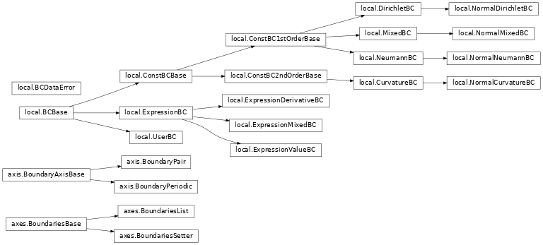
4.3.1.2 Boundaries overview
The boundaries package defines the following classes:
Local boundary conditions:
DirichletBC: Imposing a constant value of the field at the boundaryExpressionValueBC: Imposing the value of the field at the boundary given by an expression or a python functionNeumannBC: Imposing a constant derivative of the field in the outward normal direction at the boundaryExpressionDerivativeBC: Imposing the derivative of the field in the outward normal direction at the boundary given by an expression or a python functionMixedBC: Imposing the derivative of the field in the outward normal direction proportional to its value at the boundaryExpressionMixedBC: Imposing the derivative of the field in the outward normal direction proportional to its value at the boundary with coefficients given by expressions or python functionsCurvatureBC: Imposing a constant second derivative (curvature) of the field at the boundary
There are corresponding classes that only affect the normal component of a field, which
can be useful when dealing with vector and tensor fields:
NormalDirichletBC,
NormalNeumannBC,
NormalMixedBC, and
NormalCurvatureBC.
Boundaries for an axis:
BoundaryPair: Uses the local boundary conditions to specify the two boundaries along an axisBoundaryPeriodic: Indicates that an axis has periodic boundary conditions
BoundariesList for all axes of a grid:
BoundariesList: Collection of boundaries to describe conditions for all axesBoundariesSetter: Describes custom function setting virtual points to impose boundary conditions
Inheritance structure of the classes:
The details of the classes are explained below: