3.5 Performance
3.5.1 Measuring performance
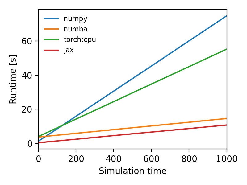
Performance of solving the Cahn-Hilliard equation with various backends.
The performance of the py-pde package depends on many details and general
statements are thus difficult to make.
However, since the core operators can be compiled using numba or torch,
many operations of the package proceed at performances close to most compiled
languages.
For a simple test case, consider the plot on the right, which shows how much real time
passed until a certain simulation time was reached.
Here, the slope of the curve quantifies the raw speed of the solver, whereas the
intercept with the y-axis indicates the start-up time, which is mainly dominated by the
compilation of the code.
The trade-off between compilation time and run time varies between backends and will
also depend on details of the simulation.
A more microscopic performance measurement concerns the actual operators, which can also be compiled using various backends. Generally, a simple Laplace operator applied to fields defined on a Cartesian grid has performance that is similar to the operators supplied by the OpenCV package. The following figures illustrate this by showing the duration of evaluating the Laplacian on grids of increasing number of support points for two different boundary conditions (lower duration is better):

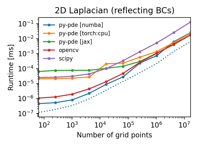
Note that the call overhead is generally lower in the py-pde package, so that the
performance on small grids is particularly good using the numba backend (blue line).
Moreover, further speed-up is possible (blue dotted line) if boundary conditions do not
need to be set, i.e., if ghost cells were set by some other function before.
However, realistic use cases probably need more complicated operations and it is
thus always necessary to profile the respective code.
This can be done using the function
estimate_computation_speed() or the traditional
timeit, profile, or even more sophisticated profilers like
pyinstrument.
3.5.2 Improving performance
Besides the underlying implementation of the operators, a major factor for performance is the specific numerical problem being solved and the methods that are used to address it. It is thus paramount to choose the right backend. Here, compiled backends, like numba and torch, provide the fastest speed, particularly for larger systems, but they require an initial compilation, which can be costly. For small systems, it can thus be advisable to use the numpy backend.
As a rule of thumb, simulations run faster when there are fewer degrees of freedom. In the case of partial differential equations, this often means using a coarser grid with fewer support points. However, there often also is an lower bound to the number of support points if structures of a certain length scales need to be resolved. Reducing the number of support points not only reduces the number of variables to be treated, but it can also allow for larger time steps. This is particularly transparent for the simple diffusion equation, where a von Neumann stability analysis reveals that the maximal time step scales as one over the discretization length squared! Choosing the right time step obviously also affects performance of a simulation. The package supports automatic choice of suitable time steps, using adaptive stepping schemes. To enable those, simply specify this in the solver call:
eq.solve(t_range=10, adaptive=True)
An initial time step can be supplied, but is not necessary.
Additional factors influencing the performance of the package include the compiler used
for numpy, scipy, and of course numba.
Performance of compiled backends, such as numba, jax, or torch, can vary
tremendously depending on problem size, the chosen device, and many other details.
Moreover, the BLAS and LAPACK libraries might make a difference.
The package has some basic support for multithreading, which can be accelerated
using the Threading Building Blocks library.
Finally, it can help to install the intel short vector math library (SVML).
However, this is not distributed with macports and might thus be more
difficult to enable.
Using macports, one could for instance install the following variants of typical packages
port install py312-numpy +gcc14+openblas
port install py312-scipy +gcc14+openblas
port install py312-numba +tbb
Note that you can disable the automatic multithreading via Configuration parameters.
Note that many details of the installed packages can affect performance and one should thus test various options if speed is critical. The suggestions above might also already be outdated.
3.5.3 Multiprocessing using MPI
The package also supports parallel simulations of PDEs using the Message Passing
Interface (MPI), which
allows combining the power of CPU cores that do not share memory. To use this advanced
simulation technique, a working implementation of MPI needs to be installed on the
computer. Usually, this is done automatically, when the optional package
numba-mpi is installed via pip or conda.
To run simulations in parallel, the special solver
ExplicitMPISolver needs to be used and the entire
script needs to be started using mpiexec.
Taken together, a minimal example reads
from pde import DiffusionPDE, ScalarField, UnitGrid

grid = UnitGrid([64, 64])
state = ScalarField.random_uniform(grid, 0.2, 0.3)

eq = DiffusionPDE(diffusivity=0.1)
result = eq.solve(state, t_range=10, dt=0.1, solver="explicit_mpi")

if result is not None:  # restrict the output to the main node
   result.plot()
Saving this script as multiprocessing.py, we can evoke a parallel simulation using
mpiexec -n 2 python3 multiprocessing.py
Here, the number 2 determines the number of cores that will be used.
Note that macOS might require an additional hint on how to connect the processes even
when they are run on the same machine (e.g., your workstation). It might help to run
mpiexec -n 2 -host localhost:2 python3 multiprocessing.py in this case.
In the example above, two python processes will start in parallel and run independently at first. In particular, both processes will load all packages and create the initial state field as well as the PDE class eq. Once the explicit_mpi solver is evoked, the processes will start communicating. py-pde will split up the full grid into two sub-grids, in this case of shape 32x64, distribute the associated sub-fields to both processes and ask each process to evolve the PDE for their sub-field. Note that boundary conditions are treated and boundary values are exchanged between neighboring sub-grids automatically. To avoid confusion, trackers will only be used on one process and also the result is only returned in one process to avoid problems where multiple process write data simultaneously. Consequently, the example above checked whether result is None (in which case the corresponding process is a child process) and only resumes analysis when the result is actually present.
The automatic treatment tries to use sensible default values, so typical simulations
work out of the box.
However, in some situations it might be advantageous to adjust these values.
For instance, the decomposition of the grid can be affected by an argument
decomposition, which can be passed to the solve() method
or the ExplicitMPISolver.
The argument should be a list with one integer for each axis in the grid, which
specifies how often the particular axis is divided.
Warning
The automatic division of the grid into sub-grids can lead to unexpected behavior,
particularly in custom PDEs that were not designed for this use case.
As a rule of thumb, all local operations are fine (since they can be performed on
each subgrid), while global operations might need synchronization between all
subgrids. One example is integration, which has been implemented properly in py-pde.
Consequently, it is safe to use integral.