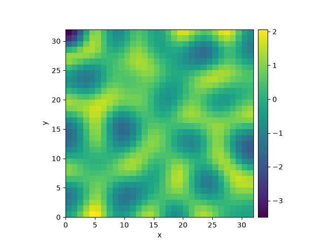
2.19 Kuramoto-Sivashinsky - Using custom class

This example implements a scalar PDE using a custom class. We here consider the Kuramoto–Sivashinsky equation, which for instance describes the dynamics of flame fronts:

\[\partial_t u = -\frac12 |\nabla u|^2 - \nabla^2 u - \nabla^4 u\]

  0%|          | 0/10.0 [00:00<?, ?it/s]
Initializing:   0%|          | 0/10.0 [00:00<?, ?it/s]
  0%|          | 0/10.0 [00:00<?, ?it/s]
  3%|▎         | 0.26/10.0 [00:00<00:13,  1.39s/it]
  7%|▋         | 0.67/10.0 [00:00<00:05,  1.66it/s]
 27%|██▋       | 2.69/10.0 [00:00<00:01,  4.37it/s]
 71%|███████   | 7.08/10.0 [00:01<00:00,  6.61it/s]
 71%|███████   | 7.08/10.0 [00:01<00:00,  5.15it/s]
100%|██████████| 10.0/10.0 [00:01<00:00,  7.27it/s]
100%|██████████| 10.0/10.0 [00:01<00:00,  7.27it/s]

from pde import PDEBase, ScalarField, UnitGrid


class KuramotoSivashinskyPDE(PDEBase):
    """Implementation of the normalized Kuramoto–Sivashinsky equation"""

    def evolution_rate(self, state, t=0):
        """implement the python version of the evolution equation"""
        state_lap = state.laplace(bc="auto_periodic_neumann")
        state_lap2 = state_lap.laplace(bc="auto_periodic_neumann")
        state_grad = state.gradient(bc="auto_periodic_neumann")
        return -state_grad.to_scalar("squared_sum") / 2 - state_lap - state_lap2


grid = UnitGrid([32, 32])  # generate grid
state = ScalarField.random_uniform(grid)  # generate initial condition

eq = KuramotoSivashinskyPDE()  # define the pde
result = eq.solve(state, t_range=10, dt=0.01)
result.plot()