Note
Go to the end to download the full example code
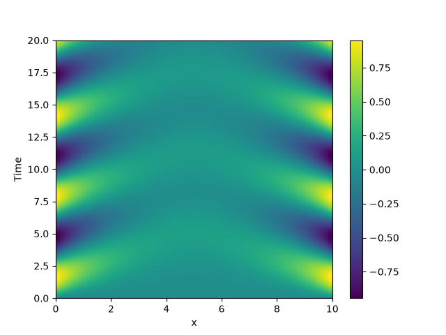
2.10 Time-dependent boundary conditions
This example solves a simple diffusion equation in one dimensions with time-dependent boundary conditions.
from pde import PDE, CartesianGrid, MemoryStorage, ScalarField, plot_kymograph

grid = CartesianGrid([[0, 10]], [64])  # generate grid
state = ScalarField(grid)  # generate initial condition

eq = PDE({"c": "laplace(c)"}, bc={"value_expression": "sin(t)"})

storage = MemoryStorage()
eq.solve(state, t_range=20, dt=1e-4, tracker=storage.tracker(0.1))

# plot the trajectory as a space-time plot
plot_kymograph(storage)
Total running time of the script: (0 minutes 8.808 seconds)