2.2.4 Multiplicative noise

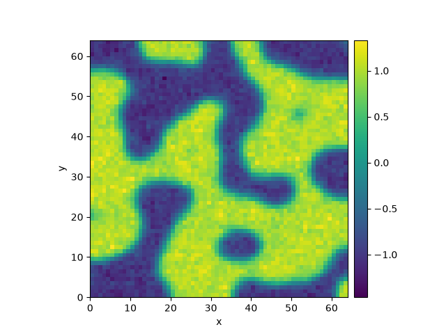
This example solves an Allen-Cahn equation where the variance of the noise depends on the field itself. Since the variance is given as an expression, its derivative is determined automatically, so the equation can be interpreted in the anti-Itô sense and integrated using the Milstein solver.

  0%|          | 0/10.0 [00:00<?, ?it/s]
Initializing:   0%|          | 0/10.0 [00:00<?, ?it/s]
  0%|          | 0/10.0 [00:06<?, ?it/s]
  0%|          | 0.004/10.0 [00:06<4:16:25, 1539.18s/it]
  1%|          | 0.119/10.0 [00:06<08:33, 51.97s/it]
  8%|▊         | 0.819/10.0 [00:06<01:11,  7.75s/it]
 25%|██▌       | 2.542/10.0 [00:06<00:19,  2.66s/it]
 53%|█████▎    | 5.257/10.0 [00:07<00:06,  1.41s/it]
 87%|████████▋ | 8.663/10.0 [00:08<00:01,  1.06it/s]
 87%|████████▋ | 8.663/10.0 [00:08<00:01,  1.02it/s]
100%|██████████| 10.0/10.0 [00:08<00:00,  1.18it/s]
100%|██████████| 10.0/10.0 [00:08<00:00,  1.18it/s]

from pde import PDE, ScalarField, UnitGrid

eq = PDE(
    {"c": "laplace(c) + c - c**3"},
    noise={"c": "0.1 * c**2"},
    noise_interpretation="anti-ito",
)
state = ScalarField.random_uniform(UnitGrid([64, 64]), -1, 1)
result = eq.solve(state, t_range=10, dt=1e-3, solver="milstein")
result.plot()