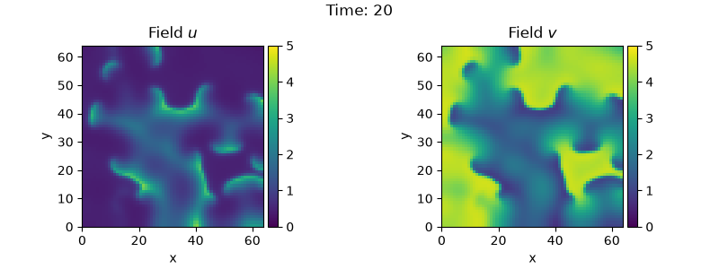
2.4.4 Brusselator - Using the ReactionDiffusionPDE class

This example uses the ReactionDiffusionPDE class to implement the Brusselator with spatial coupling,

\[\begin{split}\partial_t u &= D_0 \nabla^2 u + a - (1 + b) u + v u^2 \\ \partial_t v &= D_1 \nabla^2 v + b u - v u^2\end{split}\]

Here, \(D_0\) and \(D_1\) are the respective diffusivity and the parameters \(a\) and \(b\) are related to reaction rates.

Note that the PDE can also be implemented using the PDE class; see the example.

from pde import (
    FieldCollection,
    PlotTracker,
    ReactionDiffusionPDE,
    ScalarField,
    UnitGrid,
)

# define the PDE
a, b = 1, 3
d0, d1 = 1, 0.1
eq = ReactionDiffusionPDE(
    variables=["u", "v"],
    diffusivity=[d0, d1],
    sources=[f"{a} - ({b} + 1) * u + u**2 * v", f"{b} * u - u**2 * v"],
)

# initialize state
grid = UnitGrid([64, 64])
u = ScalarField(grid, a, label="Field $u$")
v = b / a + 0.1 * ScalarField.random_normal(grid, label="Field $v$")
state = FieldCollection([u, v])

# simulate the pde
tracker = PlotTracker(interrupts=1, plot_args={"vmin": 0, "vmax": 5})
sol = eq.solve(state, t_range=20, dt=1e-3, tracker=tracker)