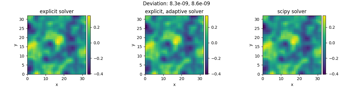
2.24. Solver comparison

This example shows how to set up solvers explicitly and how to extract diagnostic information.

/home/docs/checkouts/readthedocs.org/user_builds/py-pde/checkouts/0.29.0/pde/grids/boundaries/local.py:1822: NumbaDeprecationWarning: The 'nopython' keyword argument was not supplied to the 'numba.jit' decorator. The implicit default value for this argument is currently False, but it will be changed to True in Numba 0.59.0. See https://numba.readthedocs.io/en/stable/reference/deprecation.html#deprecation-of-object-mode-fall-back-behaviour-when-using-jit for details.
  def virtual_point(
Diagnostic information from first run:
{'controller': {'t_start': 0, 't_end': 1.0, 'profiler': {'solver': 0.0610781050000071, 'tracker': 6.172899998091452e-05, 'compilation': 5.157592117999997}, 'jit_count': {'make_stepper': 6, 'simulation': 0}, 'solver_start': '2023-05-03 09:03:38.961394', 'successful': True, 'stop_reason': 'Reached final time', 'solver_duration': '0:00:00.061138', 't_final': 1.0, 'process_count': 1}, 'package_version': 'unknown', 'solver': {'class': 'ExplicitSolver', 'pde_class': 'DiffusionPDE', 'dt': 0.001, 'steps': 1000, 'scheme': 'euler', 'state_modifications': 0.0, 'backend': 'numba', 'stochastic': False, 'dt_adaptive': False}}

Diagnostic information from second run:
{'controller': {'t_start': 0, 't_end': 1.0, 'profiler': {'solver': 0.2164038669999968, 'tracker': 5.7314000002861576e-05, 'compilation': 1.1781981660000156}, 'jit_count': {'make_stepper': 2, 'simulation': 0}, 'solver_start': '2023-05-03 09:03:40.201492', 'successful': True, 'stop_reason': 'Reached final time', 'solver_duration': '0:00:00.216485', 't_final': 1.0, 'process_count': 1}, 'package_version': 'unknown', 'solver': {'class': 'ExplicitSolver', 'pde_class': 'DiffusionPDE', 'dt': 0.001, 'steps': 26, 'scheme': 'runge-kutta', 'state_modifications': 0.0, 'dt_statistics': {'min': 0.001, 'max': 0.07639018327438296, 'mean': 0.038461538461538464, 'std': 0.019567719801290448, 'count': 26.0}, 'stochastic': False, 'backend': 'numba', 'dt_adaptive': True}}

Diagnostic information from third run:
{'controller': {'t_start': 0, 't_end': 1.0, 'profiler': {'solver': 0.003493340999995098, 'tracker': 5.7644000008849616e-05, 'compilation': 0.5952558520000082}, 'jit_count': {'make_stepper': 1, 'simulation': 0}, 'solver_start': '2023-05-03 09:03:42.510736', 'successful': True, 'stop_reason': 'Reached final time', 'solver_duration': '0:00:00.003622', 't_final': 1.0, 'process_count': 1}, 'package_version': 'unknown', 'solver': {'class': 'ScipySolver', 'pde_class': 'DiffusionPDE', 'dt': None, 'steps': 50, 'stochastic': False, 'backend': 'numba'}}

import pde

# initialize the grid, an initial condition, and the PDE
grid = pde.UnitGrid([32, 32])
field = pde.ScalarField.random_uniform(grid, -1, 1)
eq = pde.DiffusionPDE()

# try the explicit solver
solver1 = pde.ExplicitSolver(eq)
controller1 = pde.Controller(solver1, t_range=1, tracker=None)
sol1 = controller1.run(field, dt=1e-3)
sol1.label = "explicit solver"
print("Diagnostic information from first run:")
print(controller1.diagnostics)
print()

# try an explicit solver with adaptive time steps
solver2 = pde.ExplicitSolver(eq, scheme="runge-kutta", adaptive=True)
controller2 = pde.Controller(solver2, t_range=1, tracker=None)
sol2 = controller2.run(field, dt=1e-3)
sol2.label = "explicit, adaptive solver"
print("Diagnostic information from second run:")
print(controller2.diagnostics)
print()

# try the standard scipy solver
solver3 = pde.ScipySolver(eq)
controller3 = pde.Controller(solver3, t_range=1, tracker=None)
sol3 = controller3.run(field)
sol3.label = "scipy solver"
print("Diagnostic information from third run:")
print(controller3.diagnostics)
print()

# plot both fields and give the deviation as the title
title = f"Deviation: {((sol1 - sol2)**2).average:.2g}, {((sol1 - sol3)**2).average:.2g}"
pde.FieldCollection([sol1, sol2, sol3]).plot(title=title)