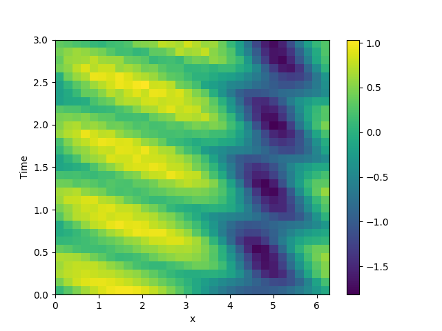
2.12. 1D problem - Using PDE class

This example implements a PDE that is only defined in one dimension. Here, we chose the Korteweg-de Vries equation, given by

\[\partial_t \phi = 6 \phi \partial_x \phi - \partial_x^3 \phi\]

which we implement using the PDE.

/home/docs/checkouts/readthedocs.org/user_builds/py-pde/checkouts/0.29.0/pde/grids/boundaries/local.py:1822: NumbaDeprecationWarning: The 'nopython' keyword argument was not supplied to the 'numba.jit' decorator. The implicit default value for this argument is currently False, but it will be changed to True in Numba 0.59.0. See https://numba.readthedocs.io/en/stable/reference/deprecation.html#deprecation-of-object-mode-fall-back-behaviour-when-using-jit for details.
  def virtual_point(

from math import pi

from pde import PDE, CartesianGrid, MemoryStorage, ScalarField, plot_kymograph

# initialize the equation and the space
eq = PDE({"φ": "6 * φ * d_dx(φ) - laplace(d_dx(φ))"})
grid = CartesianGrid([[0, 2 * pi]], [32], periodic=True)
state = ScalarField.from_expression(grid, "sin(x)")

# solve the equation and store the trajectory
storage = MemoryStorage()
eq.solve(state, t_range=3, tracker=storage.tracker(0.1))

# plot the trajectory as a space-time plot
plot_kymograph(storage)