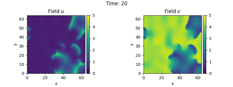
2.14. Brusselator - Using the PDE class

This example uses the PDE class to implement the Brusselator with spatial coupling,

\[\begin{split}\partial_t u &= D_0 \nabla^2 u + a - (1 + b) u + v u^2 \\ \partial_t v &= D_1 \nabla^2 v + b u - v u^2\end{split}\]

Here, \(D_0\) and \(D_1\) are the respective diffusivity and the parameters \(a\) and \(b\) are related to reaction rates.

Note that the same result can also be achieved with a full implementation of a custom class, which allows for more flexibility at the cost of code complexity.

/home/docs/checkouts/readthedocs.org/user_builds/py-pde/checkouts/0.29.0/pde/grids/boundaries/local.py:1822: NumbaDeprecationWarning: The 'nopython' keyword argument was not supplied to the 'numba.jit' decorator. The implicit default value for this argument is currently False, but it will be changed to True in Numba 0.59.0. See https://numba.readthedocs.io/en/stable/reference/deprecation.html#deprecation-of-object-mode-fall-back-behaviour-when-using-jit for details.
  def virtual_point(

from pde import PDE, FieldCollection, PlotTracker, ScalarField, UnitGrid

# define the PDE
a, b = 1, 3
d0, d1 = 1, 0.1
eq = PDE(
    {
        "u": f"{d0} * laplace(u) + {a} - ({b} + 1) * u + u**2 * v",
        "v": f"{d1} * laplace(v) + {b} * u - u**2 * v",
    }
)

# initialize state
grid = UnitGrid([64, 64])
u = ScalarField(grid, a, label="Field $u$")
v = b / a + 0.1 * ScalarField.random_normal(grid, label="Field $v$")
state = FieldCollection([u, v])

# simulate the pde
tracker = PlotTracker(interval=1, plot_args={"vmin": 0, "vmax": 5})
sol = eq.solve(state, t_range=20, dt=1e-3, tracker=tracker)