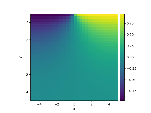
2.13. Heterogeneous boundary conditions

This example implements a spatially coupled SIR model with the following dynamics for the density of susceptible, infected, and recovered individuals:

\[\begin{split}\partial_t s &= D \nabla^2 s - \beta is \\ \partial_t i &= D \nabla^2 i + \beta is - \gamma i \\ \partial_t r &= D \nabla^2 r + \gamma i\end{split}\]

Here, \(D\) is the diffusivity, \(\beta\) the infection rate, and \(\gamma\) the recovery rate.

  0%|          | 0/10.0 [00:00<?, ?it/s]
Initializing:   0%|          | 0/10.0 [00:00<?, ?it/s]
  0%|          | 0/10.0 [00:00<?, ?it/s]
  2%|2         | 0.23/10.0 [00:00<00:09,  1.00s/it]
  7%|7         | 0.71/10.0 [00:00<00:03,  2.57it/s]
 29%|##9       | 2.94/10.0 [00:00<00:01,  6.25it/s]
 80%|########  | 8.02/10.0 [00:00<00:00,  8.84it/s]
 80%|########  | 8.02/10.0 [00:01<00:00,  7.43it/s]
100%|##########| 10.0/10.0 [00:01<00:00,  9.26it/s]
100%|##########| 10.0/10.0 [00:01<00:00,  9.26it/s]

import numpy as np

from pde import CartesianGrid, DiffusionPDE, ScalarField

# define grid and an initial state
grid = CartesianGrid([[-5, 5], [-5, 5]], 32)
field = ScalarField(grid)


# define the boundary conditions, which here are calculated from a function
def bc_value(adjacent_value, dx, x, y, t):
    """return boundary value"""
    return np.sign(x)


bc_x = "derivative"
bc_y = ["derivative", {"value_expression": bc_value}]

# define and solve a simple diffusion equation
eq = DiffusionPDE(bc=[bc_x, bc_y])
res = eq.solve(field, t_range=10, dt=0.01, backend="numpy")
res.plot()