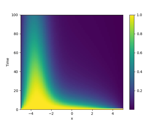
2.16. Diffusion equation with spatial dependence

This example solve the Diffusion equation with a heterogeneous diffusivity:

\[\partial_t c = \nabla\bigr( D(\boldsymbol r) \nabla c \bigr)\]

using the PDE class. In particular, we consider \(D(x) = 1.01 + \tanh(x)\), which gives a low diffusivity on the left side of the domain.

Note that the naive implementation, PDE({"c": "divergence((1.01 + tanh(x)) * gradient(c))"}), has numerical instabilities. This is because two finite difference approximations are nested. To arrive at a more stable numerical scheme, it is advisable to expand the divergence,

\[\partial_t c = D \nabla^2 c + \nabla D . \nabla c\]

/home/docs/checkouts/readthedocs.org/user_builds/py-pde/checkouts/0.29.0/pde/grids/boundaries/local.py:1822: NumbaDeprecationWarning: The 'nopython' keyword argument was not supplied to the 'numba.jit' decorator. The implicit default value for this argument is currently False, but it will be changed to True in Numba 0.59.0. See https://numba.readthedocs.io/en/stable/reference/deprecation.html#deprecation-of-object-mode-fall-back-behaviour-when-using-jit for details.
  def virtual_point(

from pde import PDE, CartesianGrid, MemoryStorage, ScalarField, plot_kymograph

# Expanded definition of the PDE
diffusivity = "1.01 + tanh(x)"
term_1 = f"({diffusivity}) * laplace(c)"
term_2 = f"dot(gradient({diffusivity}), gradient(c))"
eq = PDE({"c": f"{term_1} + {term_2}"}, bc={"value": 0})


grid = CartesianGrid([[-5, 5]], 64)  # generate grid
field = ScalarField(grid, 1)  # generate initial condition

storage = MemoryStorage()  # store intermediate information of the simulation
res = eq.solve(field, 100, dt=1e-3, tracker=storage.tracker(1))  # solve the PDE

plot_kymograph(storage)  # visualize the result in a space-time plot