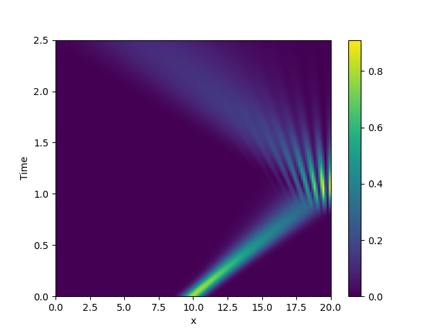
2.18. Schrödinger’s Equation

This example implements a complex PDE using the PDE. We here chose the Schrödinger equation without a spatial potential in non-dimensional form:

\[i \partial_t \psi = -\nabla^2 \psi\]

Note that the example imposes Neumann conditions at the wall, so the wave packet is expected to reflect off the wall.

/home/docs/checkouts/readthedocs.org/user_builds/py-pde/checkouts/0.29.0/pde/grids/boundaries/local.py:1822: NumbaDeprecationWarning: The 'nopython' keyword argument was not supplied to the 'numba.jit' decorator. The implicit default value for this argument is currently False, but it will be changed to True in Numba 0.59.0. See https://numba.readthedocs.io/en/stable/reference/deprecation.html#deprecation-of-object-mode-fall-back-behaviour-when-using-jit for details.
  def virtual_point(

from math import sqrt

from pde import PDE, CartesianGrid, MemoryStorage, ScalarField, plot_kymograph

grid = CartesianGrid([[0, 20]], 128, periodic=False)  # generate grid

# create a (normalized) wave packet with a certain form as an initial condition
initial_state = ScalarField.from_expression(grid, "exp(I * 5 * x) * exp(-(x - 10)**2)")
initial_state /= sqrt(initial_state.to_scalar("norm_squared").integral.real)

eq = PDE({"ψ": f"I * laplace(ψ)"})  # define the pde

# solve the pde and store intermediate data
storage = MemoryStorage()
eq.solve(initial_state, t_range=2.5, dt=1e-5, tracker=[storage.tracker(0.02)])

# visualize the results as a space-time plot
plot_kymograph(storage, scalar="norm_squared")