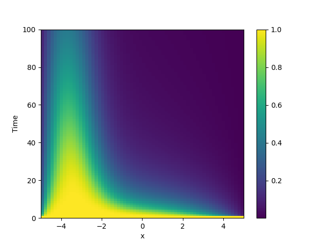
2.2.12 Diffusion equation with spatial dependence

This example solve the Diffusion equation with a heterogeneous diffusivity:

\[\partial_t c = \nabla\bigr( D(\boldsymbol r) \nabla c \bigr)\]

using the PDE class. In particular, we consider \(D(x) = 1.01 + \tanh(x)\), which gives a low diffusivity on the left side of the domain.

Note that the naive implementation, PDE({"c": "divergence((1.01 + tanh(x)) * gradient(c))"}), has numerical instabilities. This is because two finite difference approximations are nested. To arrive at a more stable numerical scheme, it is advisable to expand the divergence,

\[\partial_t c = D \nabla^2 c + \nabla D . \nabla c\]

from pde import PDE, CartesianGrid, MemoryStorage, ScalarField, plot_kymograph

# Expanded definition of the PDE
diffusivity = "1.01 + tanh(x)"
term_1 = f"({diffusivity}) * laplace(c)"
term_2 = f"dot(gradient({diffusivity}), gradient(c))"
eq = PDE({"c": f"{term_1} + {term_2}"}, bc={"value": 0})


grid = CartesianGrid([[-5, 5]], 64)  # generate grid
field = ScalarField(grid, 1)  # generate initial condition

storage = MemoryStorage()  # store intermediate information of the simulation
res = eq.solve(field, 100, dt=1e-3, tracker=storage.tracker(1))  # solve the PDE

plot_kymograph(storage)  # visualize the result in a space-time plot