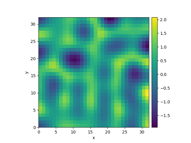
2.4.7 Kuramoto-Sivashinsky - Compiled methods

This example implements a scalar PDE using a custom class with a numba-compiled method for accelerated calculations. We here consider the Kuramoto–Sivashinsky equation, which for instance describes the dynamics of flame fronts:

\[\partial_t u = -\frac12 |\nabla u|^2 - \nabla^2 u - \nabla^4 u\]

  0%|          | 0/10.0 [00:00<?, ?it/s]
Initializing:   0%|          | 0/10.0 [00:00<?, ?it/s]
  0%|          | 0/10.0 [00:09<?, ?it/s]
  0%|          | 0.01/10.0 [00:11<3:04:42, 1109.36s/it]
  0%|          | 0.02/10.0 [00:11<1:32:15, 554.69s/it]
  2%|▏         | 0.21/10.0 [00:11<08:37, 52.83s/it]
 90%|█████████ | 9.05/10.0 [00:11<00:01,  1.23s/it]
 90%|█████████ | 9.05/10.0 [00:11<00:01,  1.23s/it]
100%|██████████| 10.0/10.0 [00:11<00:00,  1.11s/it]
100%|██████████| 10.0/10.0 [00:11<00:00,  1.11s/it]

import numba as nb

from pde import PDEBase, ScalarField, UnitGrid


class KuramotoSivashinskyPDE(PDEBase):
    """Implementation of the normalized Kuramoto–Sivashinsky equation."""

    def __init__(self, bc="auto_periodic_neumann"):
        super().__init__()
        self.bc = bc

    def evolution_rate(self, state, t=0):
        """Implement the python version of the evolution equation."""
        state_lap = state.laplace(bc=self.bc)
        state_lap2 = state_lap.laplace(bc=self.bc)
        state_grad_sq = state.gradient_squared(bc=self.bc)
        return -state_grad_sq / 2 - state_lap - state_lap2

    def _make_pde_rhs_numba(self, state):
        """Nunmba-compiled implementation of the PDE."""
        gradient_squared = state.grid.make_operator("gradient_squared", bc=self.bc)
        laplace = state.grid.make_operator("laplace", bc=self.bc)

        @nb.njit
        def pde_rhs(data, t):
            return -0.5 * gradient_squared(data) - laplace(data + laplace(data))

        return pde_rhs


grid = UnitGrid([32, 32])  # generate grid
state = ScalarField.random_uniform(grid)  # generate initial condition

eq = KuramotoSivashinskyPDE()  # define the pde
result = eq.solve(state, t_range=10, dt=0.01)
result.plot()