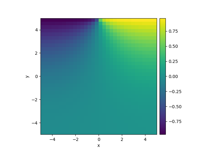
2.4.2 Heterogeneous boundary conditions

This example implements a diffusion equation with a boundary condition specified by a function, which can in principle depend on time.

  0%|          | 0/10.0 [00:00<?, ?it/s]
Initializing:   0%|          | 0/10.0 [00:00<?, ?it/s]
  0%|          | 0/10.0 [00:00<?, ?it/s]
  3%|▎         | 0.32/10.0 [00:00<00:03,  2.96it/s]
 13%|█▎        | 1.28/10.0 [00:00<00:00,  8.77it/s]
 62%|██████▏   | 6.22/10.0 [00:00<00:00, 18.49it/s]
 62%|██████▏   | 6.22/10.0 [00:00<00:00, 12.91it/s]
100%|██████████| 10.0/10.0 [00:00<00:00, 20.74it/s]
100%|██████████| 10.0/10.0 [00:00<00:00, 20.74it/s]

import numpy as np

from pde import CartesianGrid, DiffusionPDE, ScalarField

# define grid and an initial state
grid = CartesianGrid([[-5, 5], [-5, 5]], 32)
field = ScalarField(grid)


# define the boundary conditions, which here are calculated from a function
def bc_value(adjacent_value, dx, x, y, t):
    """Return boundary value."""
    return np.sign(x)


# define and solve a simple diffusion equation
eq = DiffusionPDE(bc={"*": {"derivative": 0}, "y+": {"value_expression": bc_value}})
res = eq.solve(field, t_range=10, dt=0.01, backend="numpy")
res.plot()