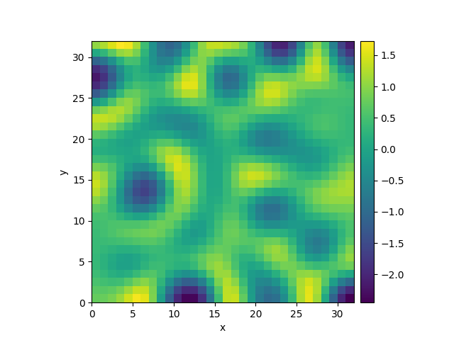
2.6. Kuramoto-Sivashinsky - Using PDE class

This example implements a scalar PDE using the PDE. We here consider the Kuramoto–Sivashinsky equation, which for instance describes the dynamics of flame fronts:

\[\partial_t u = -\frac12 |\nabla u|^2 - \nabla^2 u - \nabla^4 u\]

  0%|          | 0/10.0 [00:00<?, ?it/s]
Initializing:   0%|          | 0/10.0 [00:00<?, ?it/s]/home/docs/checkouts/readthedocs.org/user_builds/py-pde/checkouts/0.30.0/pde/grids/boundaries/local.py:1822: NumbaDeprecationWarning: The 'nopython' keyword argument was not supplied to the 'numba.jit' decorator. The implicit default value for this argument is currently False, but it will be changed to True in Numba 0.59.0. See https://numba.readthedocs.io/en/stable/reference/deprecation.html#deprecation-of-object-mode-fall-back-behaviour-when-using-jit for details.
  def virtual_point(

  0%|          | 0/10.0 [00:15<?, ?it/s]
  0%|          | 0.01/10.0 [00:27<7:42:09, 2775.72s/it]
  0%|          | 0.02/10.0 [00:27<3:50:51, 1387.88s/it]
  1%|1         | 0.11/10.0 [00:27<41:35, 252.35s/it]
 44%|####4     | 4.45/10.0 [00:27<00:34,  6.24s/it]
 44%|####4     | 4.45/10.0 [00:27<00:34,  6.24s/it]
100%|##########| 10.0/10.0 [00:27<00:00,  2.78s/it]
100%|##########| 10.0/10.0 [00:27<00:00,  2.78s/it]

from pde import PDE, ScalarField, UnitGrid

grid = UnitGrid([32, 32])  # generate grid
state = ScalarField.random_uniform(grid)  # generate initial condition

eq = PDE({"u": "-gradient_squared(u) / 2 - laplace(u + laplace(u))"})  # define the pde
result = eq.solve(state, t_range=10, dt=0.01)
result.plot()