4.2 pde.fields package
Package defining fields, which contain the actual data stored on discrete grids.
Scalar field discretized on a grid. |
|
Vector field discretized on a grid. |
|
Tensor field of rank 2 discretized on a grid. |
|
Collection of fields defined on the same grid. |
Inheritance structure of the classes:
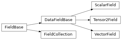
The details of the classes are explained below:
- class FieldCollection(fields, *, copy_fields=False, label=None, labels=None, dtype=None)[source]
Bases:
FieldBaseCollection of fields defined on the same grid.
Note
All fields in a collection must have the same data type. This might lead to up-casting, where for instance a combination of a real-valued and a complex-valued field will be both stored as complex fields.
- Parameters:
fields (sequence or mapping of
DataFieldBase) – Sequence or mapping of the individual fields. If a mapping is used, the keys set the names of the individual fields.copy_fields (bool) – Flag determining whether the individual fields given in fields are copied. Note that fields are always copied if some of the supplied fields are identical. If fields are copied the original fields will be left untouched. Conversely, if copy_fields == False, the original fields are modified so their data points to the collection. It is thus basically impossible to have fields that are linked to multiple collections at the same time.
label (str) – Label of the field collection
labels (list of str) – Labels of the individual fields. If omitted, the labels from the fields argument are used.
dtype (numpy dtype) – The data type of the field. All the numpy dtypes are supported. If omitted, it will be determined from data automatically.
- append(*fields, label=None)[source]
Create new collection with appended field(s)
- Parameters:
*fields (FieldCollection or DataFieldBase) – A sequence of single fields or collection of fields that will be appended to the fields in the current collection. The data of all fields will be copied.
label (str) – Label of the new field collection. If omitted, the current label is used
- Returns:
A new field collection, which combines the current one with fields given by fields.
- Return type:
- assert_field_compatible(other, accept_scalar=False)[source]
Checks whether other is compatible with the current field.
- Parameters:
other (FieldBase) – Other field this is compared to
accept_scalar (bool, optional) – Determines whether it is acceptable that other is an instance of
ScalarField.
- copy(*, label=None, dtype=None)[source]
Return a copy of the data, but not of the grid.
- Parameters:
label (str, optional) – Name of the returned field
dtype (numpy dtype) – The data type of the field. If omitted, it will be determined from data automatically.
self (FieldCollection)
- Return type:
- property fields: list[DataFieldBase]
the fields of this collection
- Type:
- classmethod from_data(field_classes, grid, data, *, with_ghost_cells=True, label=None, labels=None, dtype=None)[source]
Create a field collection from classes and data.
- Parameters:
field_classes (list) – List of the classes that define the individual fields
data (
ndarray, optional) – Data values of all fields at support points of the gridgrid (
GridBase) – Grid defining the space on which this field is defined.with_ghost_cells (bool) – Indicates whether the ghost cells are included in data
label (str) – Label of the field collection
labels (list of str) – Labels of the individual fields. If omitted, the labels from the fields argument are used.
dtype (numpy dtype) – The data type of the field. All the numpy dtypes are supported. If omitted, it will be determined from data automatically.
- Return type:
- classmethod from_scalar_expressions(grid, expressions, *, user_funcs=None, consts=None, label=None, labels=None, dtype=None)[source]
Create a field collection on a grid from given expressions.
Warning
This implementation uses
exec()and should therefore not be used in a context where malicious input could occur.- Parameters:
grid (
GridBase) – Grid defining the space on which this field is definedexpressions (list of str) – A list of mathematical expression, one for each field in the collection. The expressions determine the values as a function of the position on the grid. The expressions may contain standard mathematical functions and they may depend on the axes labels of the grid. More information can be found in the expression documentation.
user_funcs (dict, optional) – A dictionary with user defined functions that can be used in the expression
consts (dict, optional) – A dictionary with user defined constants that can be used in the expression. The values of these constants should either be numbers or
ndarray.label (str, optional) – Name of the whole collection
labels (list of str, optional) – Names of the individual fields
dtype (numpy dtype) – The data type of the field. All the numpy dtypes are supported. If omitted, it will be determined from data automatically.
- Return type:
- classmethod from_state(attributes, data=None)[source]
Create a field collection from given state.
- Parameters:
- Return type:
- get_line_data(index=0, scalar='auto', extract='auto')[source]
Return data for a line plot of the field.
- Parameters:
- Returns:
Information useful for performing a line plot of the field
- Return type:
- interpolate_to_grid(grid, *, fill=None, label=None)[source]
Interpolate the data of this field collection to another grid.
- Parameters:
grid (
GridBase) – The grid of the new field onto which the current field is interpolated.fill (Number, optional) – Determines how values out of bounds are handled. If None, a ValueError is raised when out-of-bounds points are requested. Otherwise, the given value is returned.
label (str, optional) – Name of the returned field collection
- Returns:
Interpolated data
- Return type:
- property labels: _FieldLabels
the labels of all fields.
Note
The attribute returns a special class
_FieldLabelsto allow specific manipulations of the field labels. The returned object behaves much like a list, but assigning values will modify the labels of the fields in the collection.- Type:
_FieldLabels
- plot(kind='auto', figsize='auto', arrangement='horizontal', subplot_args=None, *args, title=None, constrained_layout=True, filename=None, action='auto', fig_style=None, fig=None, **kwargs)[source]
Visualize all the fields in the collection.
- Parameters:
kind (str or list of str) – Determines the kind of the visualizations. Supported values are image, line, vector, interactive, or merged. Alternatively, auto determines the best visualization based on each field itself. Instead of a single value for all fields, a list with individual values can be given, unless merged is chosen.
figsize (str or tuple of numbers) – Determines the figure size. The figure size is unchanged if the string default is passed. Conversely, the size is adjusted automatically when auto is passed. Finally, a specific figure size can be specified using two values, using
matplotlib.figure.Figure.set_size_inches().arrangement (str or tuple of int) – Determines how the sub panels will be arranged. The default value horizontal places all subplots next to each other, whereas vertical puts them below each other. Alternatively, an exact number of rows and columns can be specified by the tuple
(nrows, ncols). Negative values will be replaced by suitable values that ensure enough panels.subplot_args (list) – Additional arguments for the specific subplots. Should be a list with a dictionary of arguments for each subplot. Supplying an empty dict allows to keep the default setting of specific subplots.
title (str) – Title of the plot. If omitted, the title might be chosen automatically. This is shown above all panels.
constrained_layout (bool) – Whether to use constrained_layout in
matplotlib.pyplot.figure()call to create a figure. This affects the layout of all plot elements. Generally, spacing might be better with this flag enabled, but it can also lead to problems when plotting multiple plots successively, e.g., when creating a movie.filename (str, optional) – If given, the figure is written to the specified file.
action (str) – Decides what to do with the final figure. If the argument is set to show,
matplotlib.pyplot.show()will be called to show the plot. If the value is none, the figure will be created, but not necessarily shown. The value close closes the figure, after saving it to a file when filename is given. The default value auto implies that the plot is shown if it is not a nested plot call.fig_style (dict) – Dictionary with properties that will be changed on the figure after the plot has been drawn by calling
matplotlib.pyplot.setp(). For instance, using fig_style={‘dpi’: 200} increases the resolution of the figure.fig (
matplotlib.figures.Figure) – Figure that is used for plotting. If omitted, a new figure is created.**kwargs – All additional keyword arguments are forwarded to the actual plotting function of all subplots.
- Returns:
Instances that contain information to update all the plots with new data later.
- Return type:
List of
PlotReference
- project(axes, *, label=None, **kwargs)[source]
Project fields along given axes.
This is currently only implemented for scalar fields. If any field in the collection has higher rank, the entire process fails.
- Parameters:
axes (list of str) – The names of the axes that are removed by the projection operation. The valid names for a given grid are the ones in the
GridBase.axesattribute.label (str, optional) – Name of the returned collection. If omitted, the current label is used.
**kwargs – Additional arguments forwarded to the projection method (e.g., method).
- Returns:
The projected data of all fields on a subgrid of the original grid.
- Return type:
- classmethod scalar_random_uniform(num_fields, grid, vmin=0, vmax=1, *, label=None, labels=None, rng=None)[source]
Create scalar fields with random values between vmin and vmax
- Parameters:
num_fields (int) – The number of fields to create
grid (
GridBase) – Grid defining the space on which the fields are definedvmin (float) – Lower bound. Can be complex to create complex fields
vmax (float) – Upper bound. Can be complex to create complex fields
label (str, optional) – Name of the field collection
labels (list of str, optional) – Names of the individual fields
rng (
Generator) – Random number generator (default:default_rng())
- Return type:
- slice(position, *, label=None, **kwargs)[source]
Slice all fields at a given position.
This is currently only implemented for scalar fields. If any field in the collection has higher rank, the entire process fails.
- Parameters:
position (dict) – Determines the location of the slice using a dictionary supplying coordinate values for a subset of axes. Axes not mentioned in the dictionary are retained and form the slice. For instance, in a 2d Cartesian grid, position = {‘x’: 1} slices along the y-direction at x=1. Additionally, the special positions ‘low’, ‘mid’, and ‘high’ are supported to reference relative positions along the axis.
label (str, optional) – Name of the returned collection. If omitted, the current label is used.
**kwargs – Additional arguments forwarded to the slicing method (e.g., method).
- Returns:
The projected data of all fields on a subgrid of the original grid.
- Return type:
- smooth(sigma=1, *, out=None, label=None)[source]
Applies Gaussian smoothing with the given standard deviation.
This function respects periodic boundary conditions of the underlying grid, using reflection when no periodicity is specified.
- Parameters:
sigma (float) – Gives the standard deviation of the smoothing in real length units (default: 1)
out (FieldCollection, optional) – Optional field into which the smoothed data is stored
label (str, optional) – Name of the returned field
- Returns:
Smoothed data, stored at out if given.
- Return type:
- class ScalarField(grid, data='zeros', *, label=None, dtype=None, with_ghost_cells=False)[source]
Bases:
DataFieldBaseScalar field discretized on a grid.
- Parameters:
grid (
GridBase) – Grid defining the space on which this field is defined.data (Number or
ndarray, optional) – Field values at the support points of the grid. The flag with_ghost_cells determines whether this data array contains values for the ghost cells, too. The resulting field will contain real data unless the data argument contains complex values. Special values are “zeros” or None, initializing the field with zeros, and “empty”, just allocating memory with unspecified values.label (str, optional) – Name of the field
dtype (numpy dtype) – The data type of the field. If omitted, it will be determined from data automatically.
with_ghost_cells (bool) – Indicates whether the ghost cells are included in data
- classmethod from_expression(grid, expression, *, user_funcs=None, consts=None, label=None, dtype=None)[source]
Create a scalar field on a grid from a given expression.
Warning
This implementation uses
exec()and should therefore not be used in a context where malicious input could occur.- Parameters:
grid (
GridBase) – Grid defining the space on which this field is definedexpression (str) – Mathematical expression for the scalar value as a function of the position on the grid. The expression may contain standard mathematical functions and it may depend on the axes labels of the grid. More information can be found in the expression documentation.
user_funcs (dict, optional) – A dictionary with user defined functions that can be used in the expression
consts (dict, optional) – A dictionary with user defined constants that can be used in the expression. The values of these constants should either be numbers or
ndarray.label (str, optional) – Name of the field
dtype (numpy dtype) – The data type of the field. If omitted, it will be determined from data automatically.
- Return type:
- classmethod from_image(path, bounds=None, periodic=False, *, label=None)[source]
Create a scalar field from an image.
- Parameters:
path (
Pathor str) – The path to the image filebounds (tuple, optional) – Gives the coordinate range for each axis. This should be two tuples of two numbers each, which mark the lower and upper bound for each axis.
periodic (bool or list) – Specifies which axes possess periodic boundary conditions. This is either a list of booleans defining periodicity for each individual axis or a single boolean value specifying the same periodicity for all axes.
label (str, optional) – Name of the field
- Return type:
- get_boundary_field(index, bc=None, *, label=None)[source]
Get the field on the specified boundary.
- Parameters:
index (str or tuple) – Index specifying the boundary. Can be either a string given in
boundary_names, like"left", or a tuple of the axis index perpendicular to the boundary and a boolean specifying whether the boundary is at the upper side of the axis or not, e.g.,(1, True).bc (BoundariesData | None) – The boundary conditions applied to the field. Boundary conditions are generally given as a dictionary with one condition for each axis side. For periodic axes, only periodic boundary conditions are allowed (indicated by ‘periodic’ and ‘anti-periodic’). For non-periodic axes, different boundary conditions can be specified for the lower and upper end (using specific identifiers, like x- and y+). For instance, Dirichlet conditions enforcing a value NUM (specified by {‘value’: NUM}) and Neumann conditions enforcing the value DERIV for the derivative in the normal direction (specified by {‘derivative’: DERIV}) are supported. Note that the special value ‘auto_periodic_neumann’ imposes periodic boundary conditions for periodic axis and a vanishing derivative otherwise. More information can be found in the boundaries documentation. If the special value None is given, no boundary conditions are enforced. The user then needs to ensure that the ghost cells are set accordingly.
label (str) – Label of the returned field
- Returns:
The field on the boundary
- Return type:
- gradient(bc, out=None, **kwargs)[source]
Apply gradient operator and return result as a field.
- Parameters:
bc (BoundariesData | None) – The boundary conditions applied to the field. Boundary conditions are generally given as a dictionary with one condition for each axis side. For periodic axes, only periodic boundary conditions are allowed (indicated by ‘periodic’ and ‘anti-periodic’). For non-periodic axes, different boundary conditions can be specified for the lower and upper end (using specific identifiers, like x- and y+). For instance, Dirichlet conditions enforcing a value NUM (specified by {‘value’: NUM}) and Neumann conditions enforcing the value DERIV for the derivative in the normal direction (specified by {‘derivative’: DERIV}) are supported. Note that the special value ‘auto_periodic_neumann’ imposes periodic boundary conditions for periodic axis and a vanishing derivative otherwise. More information can be found in the boundaries documentation. If the special value None is given, no boundary conditions are enforced. The user then needs to ensure that the ghost cells are set accordingly.
out (pde.fields.vectorial.VectorField, optional) – Optional vector field to which the result is written.
**kwargs – Additional keyword arguments (e.g., label)
- Returns:
result of applying the operator
- Return type:
- gradient_squared(bc, out=None, **kwargs)[source]
Apply squared gradient operator and return result as a field.
This evaluates \(|\nabla \phi|^2\) for the scalar field \(\phi\)
- Parameters:
bc (BoundariesData | None) – The boundary conditions applied to the field. Boundary conditions are generally given as a dictionary with one condition for each axis side. For periodic axes, only periodic boundary conditions are allowed (indicated by ‘periodic’ and ‘anti-periodic’). For non-periodic axes, different boundary conditions can be specified for the lower and upper end (using specific identifiers, like x- and y+). For instance, Dirichlet conditions enforcing a value NUM (specified by {‘value’: NUM}) and Neumann conditions enforcing the value DERIV for the derivative in the normal direction (specified by {‘derivative’: DERIV}) are supported. Note that the special value ‘auto_periodic_neumann’ imposes periodic boundary conditions for periodic axis and a vanishing derivative otherwise. More information can be found in the boundaries documentation. If the special value None is given, no boundary conditions are enforced. The user then needs to ensure that the ghost cells are set accordingly.
out (pde.fields.scalar.ScalarField, optional) – Optional vector field to which the result is written.
**kwargs – Extra arguments are forwarded to
apply_operator()
- Returns:
the squared gradient of the field
- Return type:
- interpolate_to_grid(grid, *, bc=None, fill=None, label=None)[source]
Interpolate the data of this scalar field to another grid.
- Parameters:
grid (
GridBase) – The grid of the new field onto which the current field is interpolated.bc (BoundariesData | None) – The boundary conditions applied to the field, which affects values close to the boundary. If omitted, the argument fill is used to determine values outside the domain. Boundary conditions are generally given as a dictionary with one condition for each axis side. For periodic axes, only periodic boundary conditions are allowed (indicated by ‘periodic’ and ‘anti-periodic’). For non-periodic axes, different boundary conditions can be specified for the lower and upper end (using specific identifiers, like x- and y+). For instance, Dirichlet conditions enforcing a value NUM (specified by {‘value’: NUM}) and Neumann conditions enforcing the value DERIV for the derivative in the normal direction (specified by {‘derivative’: DERIV}) are supported. Note that the special value ‘auto_periodic_neumann’ imposes periodic boundary conditions for periodic axis and a vanishing derivative otherwise. More information can be found in the boundaries documentation. If the special value None is given, no boundary conditions are enforced. The user then needs to ensure that the ghost cells are set accordingly.
fill (Number, optional) – Determines how values out of bounds are handled. If None, a ValueError is raised when out-of-bounds points are requested. Otherwise, the given value is returned.
label (str, optional) – Name of the returned field
self (ScalarField)
- Returns:
Field of the same rank as the current one.
- Return type:
- laplace(bc, out=None, **kwargs)[source]
Apply Laplace operator and return result as a field.
- Parameters:
bc (BoundariesData | None) – The boundary conditions applied to the field. Boundary conditions are generally given as a dictionary with one condition for each axis side. For periodic axes, only periodic boundary conditions are allowed (indicated by ‘periodic’ and ‘anti-periodic’). For non-periodic axes, different boundary conditions can be specified for the lower and upper end (using specific identifiers, like x- and y+). For instance, Dirichlet conditions enforcing a value NUM (specified by {‘value’: NUM}) and Neumann conditions enforcing the value DERIV for the derivative in the normal direction (specified by {‘derivative’: DERIV}) are supported. Note that the special value ‘auto_periodic_neumann’ imposes periodic boundary conditions for periodic axis and a vanishing derivative otherwise. More information can be found in the boundaries documentation. If the special value None is given, no boundary conditions are enforced. The user then needs to ensure that the ghost cells are set accordingly.
out (pde.fields.scalar.ScalarField, optional) – Optional scalar field to which the result is written.
**kwargs – Additional keyword arguments (e.g., label)
- Returns:
the Laplacian of the field
- Return type:
- project(axes, *, method='integral', label=None)[source]
Project scalar field along given axes.
- Parameters:
axes (list of str) – The names of the axes that are removed by the projection operation. The valid names for a given grid are the ones in the
GridBase.axesattribute.method (str) – The projection method. This can be either ‘integral’ to integrate over the removed axes or ‘average’ to perform an average instead.
label (str, optional) – The label of the returned field
- Returns:
The projected data in a scalar field with a subgrid of the original grid.
- Return type:
- rank = 0
- slice(position, *, method='nearest', label=None)[source]
Slice data at a given position.
Note
This method should not be used to evaluate fields right at the boundary since it does not respect boundary conditions. Use
get_boundary_field()to obtain the values directly on the boundary.- Parameters:
position (dict) – Determines the location of the slice using a dictionary supplying coordinate values for a subset of axes. Axes not mentioned in the dictionary are retained and form the slice. For instance, in a 2d Cartesian grid, position = {‘x’: 1} slices along the y-direction at x=1. Additionally, the special positions ‘low’, ‘mid’, and ‘high’ are supported to reference relative positions along the axis.
method (str) – The method used for slicing. Currently, we only support nearest, which takes data from cells defined on the grid.
label (str, optional) – The label of the returned field
- Returns:
The sliced data in a scalar field with a subgrid of the original grid.
- Return type:
- to_scalar(scalar='auto', *, label=None)[source]
Return a modified scalar field by applying method scalar
- Parameters:
scalar (str or callable) – Determines the method used for obtaining the scalar. If this is a callable, it is simply applied to self.data and a new scalar field with this data is returned. Alternatively, pre-defined methods can be selected using strings. Here, abs and norm denote the norm of each entry of the field, while norm_squared returns the squared norm. The default auto is to return a (unchanged) copy of a real field and the norm of a complex field.
label (str, optional) – Name of the returned field
- Returns:
Scalar field after applying the operation
- Return type:
- class Tensor2Field(grid, data='zeros', *, label=None, dtype=None, with_ghost_cells=False)[source]
Bases:
DataFieldBaseTensor field of rank 2 discretized on a grid.
Warning
Components of the tensor field are given in the local basis. While the local basis is identical to the global basis in Cartesian coordinates, the local basis depends on position in curvilinear coordinate systems. Moreover, the field always contains all components, even if the underlying grid assumes symmetries.
- Parameters:
grid (
GridBase) – Grid defining the space on which this field is defined.data (Number or
ndarray, optional) – Field values at the support points of the grid. The flag with_ghost_cells determines whether this data array contains values for the ghost cells, too. The resulting field will contain real data unless the data argument contains complex values. Special values are “zeros” or None, initializing the field with zeros, and “empty”, just allocating memory with unspecified values.label (str, optional) – Name of the field
dtype (numpy dtype) – The data type of the field. If omitted, it will be determined from data automatically.
with_ghost_cells (bool) – Indicates whether the ghost cells are included in data
- convert(form, inplace=False, *, label=None)[source]
Convert tensor to a specific form in each point in space.
- Parameters:
- Returns:
converted tensor field
- Return type:
- divergence(bc, out=None, **kwargs)[source]
Apply tensor divergence and return result as a field.
The tensor divergence is a vector field \(v_\alpha\) resulting from a contracting of the derivative of the tensor field \(t_{\alpha\beta}\):
\[v_\alpha = \sum_\beta \frac{\partial t_{\alpha\beta}}{\partial x_\beta}\]- Parameters:
bc (BoundariesData | None) – The boundary conditions applied to the field. Boundary conditions are generally given as a dictionary with one condition for each axis side. For periodic axes, only periodic boundary conditions are allowed (indicated by ‘periodic’ and ‘anti-periodic’). For non-periodic axes, different boundary conditions can be specified for the lower and upper end (using specific identifiers, like x- and y+). For instance, Dirichlet conditions enforcing a value NUM (specified by {‘value’: NUM}) and Neumann conditions enforcing the value DERIV for the derivative in the normal direction (specified by {‘derivative’: DERIV}) are supported. Note that the special value ‘auto_periodic_neumann’ imposes periodic boundary conditions for periodic axis and a vanishing derivative otherwise. More information can be found in the boundaries documentation. If the special value None is given, no boundary conditions are enforced. The user then needs to ensure that the ghost cells are set accordingly.
out (pde.fields.vectorial.VectorField, optional) – Optional scalar field to which the result is written.
**kwargs – Additional arguments affecting how the operator behaves.
- Returns:
result of applying the operator
- Return type:
- dot(other: VectorField, out: VectorField | None = None, *, conjugate: bool = True, label: str = 'dot product') VectorField[source]
- dot(other: Tensor2Field, out: Tensor2Field | None = None, *, conjugate: bool = True, label: str = 'dot product') Tensor2Field
Calculate the dot product involving a tensor field.
This supports the dot product between two tensor fields as well as the product between a tensor and a vector. The resulting fields will be a tensor or vector, respectively.
- Parameters:
other (pde.fields.vectorial.VectorField or pde.fields.tensorial.Tensor2Field) – the second field
out (pde.fields.vectorial.VectorField or pde.fields.tensorial.Tensor2Field, optional) – Optional field to which the result is written.
conjugate (bool) – Whether to use the complex conjugate for the second operand
label (str, optional) – Name of the returned field
- Returns:
VectorFieldorTensor2Field: result of applying dot operator- Return type:
- classmethod from_expression(grid, expressions, *, user_funcs=None, consts=None, label=None, dtype=None)[source]
Create a tensor field on a grid from given expressions.
Warning
This implementation uses
exec()and should therefore not be used in a context where malicious input could occur.- Parameters:
grid (
GridBase) – Grid defining the space on which this field is definedexpressions (list of str) – A 2d list of mathematical expression, one for each component of the tensor field. The expressions determine the values as a function of the position on the grid. The expressions may contain standard mathematical functions and they may depend on the axes labels of the grid. More information can be found in the expression documentation.
user_funcs (dict, optional) – A dictionary with user defined functions that can be used in the expression
consts (dict, optional) – A dictionary with user defined constants that can be used in the expression. The values of these constants should either be numbers or
ndarray.label (str, optional) – Name of the field
dtype (numpy dtype) – The data type of the field. If omitted, it will be determined from data automatically.
- Return type:
- is_symmetric(rtol=1e-05, atol=1e-08)[source]
Returns whether the tensor is symmetric.
- Parameters:
rtol (float) – The relative tolerance parameter (see
allclose()).atol (float) – The absolute tolerance parameter (see
allclose()).
- Return type:
- plot_components(kind='auto', *args, title=None, constrained_layout=True, filename=None, action='auto', fig_style=None, fig=None, **kwargs)[source]
Visualize all the components of this tensor field.
- Parameters:
kind (str or list of str) – Determines the kind of the visualizations. Supported values are image or line. Alternatively, auto determines the best visualization based on the grid.
title (str) – Title of the plot. If omitted, the title might be chosen automatically. This is shown above all panels.
constrained_layout (bool) – Whether to use constrained_layout in
matplotlib.pyplot.figure()call to create a figure. This affects the layout of all plot elements. Generally, spacing might be better with this flag enabled, but it can also lead to problems when plotting multiple plots successively, e.g., when creating a movie.filename (str, optional) – If given, the figure is written to the specified file.
action (str) – Decides what to do with the final figure. If the argument is set to show,
matplotlib.pyplot.show()will be called to show the plot. If the value is none, the figure will be created, but not necessarily shown. The value close closes the figure, after saving it to a file when filename is given. The default value auto implies that the plot is shown if it is not a nested plot call.fig_style (dict) – Dictionary with properties that will be changed on the figure after the plot has been drawn by calling
matplotlib.pyplot.setp(). For instance, using fig_style={‘dpi’: 200} increases the resolution of the figure.fig (
matplotlib.figures.Figure) – Figure that is used for plotting. If omitted, a new figure is created.**kwargs – All additional keyword arguments are forwarded to the actual plotting function of all subplots.
- Returns:
Instances that contain information to update all the plots with new data later.
- Return type:
2d list of
PlotReference
- rank = 2
- symmetrize(make_traceless=False, inplace=False, *, label=None)[source]
Symmetrize the tensor field.
- Parameters:
- Returns:
result of the operation
- Return type:
- to_scalar(scalar='auto', *, label='scalar `{scalar}`')[source]
Return scalar variant of the field.
The invariants of the tensor field \(\boldsymbol{A}\) are
\[\begin{split}I_1 &= \mathrm{tr}(\boldsymbol{A}) \\ I_2 &= \frac12 \left[ (\mathrm{tr}(\boldsymbol{A})^2 - \mathrm{tr}(\boldsymbol{A}^2) \right] \\ I_3 &= \det(A)\end{split}\]where tr denotes the trace and det denotes the determinant. Note that the three invariants can only be distinct and non-zero in three dimensions. In two dimensional spaces, we have the identity \(2 I_2 = I_3\) and in one-dimensional spaces, we have \(I_1 = I_3\) as well as \(I_2 = 0\).
- Parameters:
- Returns:
the scalar field after applying the operation
- Return type:
- trace(*, label='trace')[source]
Return the trace of the tensor field as a scalar field.
- Parameters:
label (str, optional) – Name of the returned field
- Returns:
scalar field of traces
- Return type:
- class VectorField(grid, data='zeros', *, label=None, dtype=None, with_ghost_cells=False)[source]
Bases:
DataFieldBaseVector field discretized on a grid.
Warning
Components of the vector field are given in the local basis. While the local basis is identical to the global basis in Cartesian coordinates, the local basis depends on position in curvilinear coordinate systems. Moreover, the field always contains all components, even if the underlying grid assumes symmetries.
- Parameters:
grid (
GridBase) – Grid defining the space on which this field is defined.data (Number or
ndarray, optional) – Field values at the support points of the grid. The flag with_ghost_cells determines whether this data array contains values for the ghost cells, too. The resulting field will contain real data unless the data argument contains complex values. Special values are “zeros” or None, initializing the field with zeros, and “empty”, just allocating memory with unspecified values.label (str, optional) – Name of the field
dtype (numpy dtype) – The data type of the field. If omitted, it will be determined from data automatically.
with_ghost_cells (bool) – Indicates whether the ghost cells are included in data
- divergence(bc, out=None, **kwargs)[source]
Apply divergence operator and return result as a field.
- Parameters:
bc (BoundariesData | None) – The boundary conditions applied to the field. Boundary conditions are generally given as a dictionary with one condition for each axis side. For periodic axes, only periodic boundary conditions are allowed (indicated by ‘periodic’ and ‘anti-periodic’). For non-periodic axes, different boundary conditions can be specified for the lower and upper end (using specific identifiers, like x- and y+). For instance, Dirichlet conditions enforcing a value NUM (specified by {‘value’: NUM}) and Neumann conditions enforcing the value DERIV for the derivative in the normal direction (specified by {‘derivative’: DERIV}) are supported. Note that the special value ‘auto_periodic_neumann’ imposes periodic boundary conditions for periodic axis and a vanishing derivative otherwise. More information can be found in the boundaries documentation. If the special value None is given, no boundary conditions are enforced. The user then needs to ensure that the ghost cells are set accordingly.
out (pde.fields.scalar.ScalarField, optional) – Optional scalar field to which the result is written.
**kwargs – Additional arguments affecting how the operator behaves.
- Returns:
Divergence of the field
- Return type:
- dot(other: VectorField, out: ScalarField | None = None, *, conjugate: bool = True, label: str = 'dot product') ScalarField[source]
- dot(other: Tensor2Field, out: VectorField | None = None, *, conjugate: bool = True, label: str = 'dot product') VectorField
Calculate the dot product involving a vector field.
This supports the dot product between two vectors fields as well as the product between a vector and a tensor. The resulting fields will be a scalar or vector, respectively.
- Parameters:
other (
VectorFieldorTensor2Field) – the second fieldout (pde.fields.scalar.ScalarField or pde.fields.vectorial.VectorField, optional) – Optional field to which the result is written.
conjugate (bool) – Whether to use the complex conjugate for the second operand
label (str, optional) – Name of the returned field
- Returns:
ScalarFieldorVectorField: result of applying the operator- Return type:
- classmethod from_expression(grid, expressions, *, user_funcs=None, consts=None, label=None, dtype=None)[source]
Create a vector field on a grid from given expressions.
Warning
This implementation uses
exec()and should therefore not be used in a context where malicious input could occur.- Parameters:
grid (
GridBase) – Grid defining the space on which this field is definedexpressions (list of str) – A list of mathematical expression, one for each component of the vector field. The expressions determine the values as a function of the position on the grid. The expressions may contain standard mathematical functions and they may depend on the axes labels of the grid. More information can be found in the expression documentation.
user_funcs (dict, optional) – A dictionary with user defined functions that can be used in the expression
consts (dict, optional) – A dictionary with user defined constants that can be used in the expression. The values of these constants should either be numbers or
ndarray.label (str, optional) – Name of the field
dtype (numpy dtype) – The data type of the field. If omitted, it will be determined from data automatically.
- Return type:
- classmethod from_scalars(fields, *, label=None, dtype=None)[source]
Create a vector field from a list of ScalarFields.
Note that the data of the scalar fields is copied in the process
- Parameters:
- Returns:
the resulting vector field
- Return type:
- get_vector_data(transpose=False, max_points=None, **kwargs)[source]
Return data for a vector plot of the field.
- Parameters:
- Returns:
Information useful for plotting an vector field
- Return type:
- gradient(bc, out=None, **kwargs)[source]
Apply vector gradient operator and return result as a field.
The vector gradient field is a tensor field \(t_{\alpha\beta}\) that specifies the derivatives of the vector field \(v_\alpha\) with respect to all coordinates \(x_\beta\).
- Parameters:
bc (BoundariesData | None) – The boundary conditions applied to the field. Boundary conditions need to determine all components of the vector field. Boundary conditions are generally given as a dictionary with one condition for each axis side. For periodic axes, only periodic boundary conditions are allowed (indicated by ‘periodic’ and ‘anti-periodic’). For non-periodic axes, different boundary conditions can be specified for the lower and upper end (using specific identifiers, like x- and y+). For instance, Dirichlet conditions enforcing a value NUM (specified by {‘value’: NUM}) and Neumann conditions enforcing the value DERIV for the derivative in the normal direction (specified by {‘derivative’: DERIV}) are supported. Note that the special value ‘auto_periodic_neumann’ imposes periodic boundary conditions for periodic axis and a vanishing derivative otherwise. More information can be found in the boundaries documentation. If the special value None is given, no boundary conditions are enforced. The user then needs to ensure that the ghost cells are set accordingly.
out (pde.fields.vectorial.VectorField, optional) – Optional vector field to which the result is written.
**kwargs – Additional arguments affecting how the operator behaves.
- Returns:
Gradient of the field
- Return type:
- interpolate_to_grid(grid, *, bc=None, fill=None, label=None)[source]
Interpolate the data of this vector field to another grid.
- Parameters:
grid (
GridBase) – The grid of the new field onto which the current field is interpolated.bc (BoundariesData | None) – The boundary conditions applied to the field, which affects values close to the boundary. If omitted, the argument fill is used to determine values outside the domain. Boundary conditions are generally given as a dictionary with one condition for each axis side. For periodic axes, only periodic boundary conditions are allowed (indicated by ‘periodic’ and ‘anti-periodic’). For non-periodic axes, different boundary conditions can be specified for the lower and upper end (using specific identifiers, like x- and y+). For instance, Dirichlet conditions enforcing a value NUM (specified by {‘value’: NUM}) and Neumann conditions enforcing the value DERIV for the derivative in the normal direction (specified by {‘derivative’: DERIV}) are supported. Note that the special value ‘auto_periodic_neumann’ imposes periodic boundary conditions for periodic axis and a vanishing derivative otherwise. More information can be found in the boundaries documentation. If the special value None is given, no boundary conditions are enforced. The user then needs to ensure that the ghost cells are set accordingly.
fill (Number, optional) – Determines how values out of bounds are handled. If None, a ValueError is raised when out-of-bounds points are requested. Otherwise, the given value is returned.
label (str, optional) – Name of the returned field
self (VectorField)
- Returns:
Field of the same rank as the current one.
- Return type:
- laplace(bc, out=None, **kwargs)[source]
Apply vector Laplace operator and return result as a field.
The vector Laplacian is a vector field \(L_\alpha\) containing the second derivatives of the vector field \(v_\alpha\) with respect to the coordinates \(x_\beta\):
\[L_\alpha = \sum_\beta \frac{\partial^2 v_\alpha}{\partial x_\beta \partial x_\beta}\]- Parameters:
bc (BoundariesData | None) – The boundary conditions applied to the field. Boundary conditions are generally given as a dictionary with one condition for each axis side. For periodic axes, only periodic boundary conditions are allowed (indicated by ‘periodic’ and ‘anti-periodic’). For non-periodic axes, different boundary conditions can be specified for the lower and upper end (using specific identifiers, like x- and y+). For instance, Dirichlet conditions enforcing a value NUM (specified by {‘value’: NUM}) and Neumann conditions enforcing the value DERIV for the derivative in the normal direction (specified by {‘derivative’: DERIV}) are supported. Note that the special value ‘auto_periodic_neumann’ imposes periodic boundary conditions for periodic axis and a vanishing derivative otherwise. More information can be found in the boundaries documentation. If the special value None is given, no boundary conditions are enforced. The user then needs to ensure that the ghost cells are set accordingly.
out (pde.fields.vectorial.VectorField, optional) – Optional vector field to which the result is written.
**kwargs – Additional arguments affecting how the operator behaves.
- Returns:
Laplacian of the field
- Return type:
- make_outer_prod_operator(backend='numba')[source]
Return operator calculating the outer product of two vector fields.
Warning
This function does not check types or dimensions.
- Parameters:
backend (str) – The backend (e.g., ‘numba’ or ‘numba_mpi’) used for this operator.
- Returns:
function that takes two instance of
ndarray, which contain the discretized data of the two operands. An optional third argument can specify the output array to which the result is written.- Return type:
BinaryOperatorImplType
- outer_product(other, out=None, *, label=None)[source]
Calculate the outer product of this vector field with another.
- Parameters:
other (
VectorField) – The second vector fieldout (
Tensor2Field, optional) – Optional tensorial field to which the result is written.label (str, optional) – Name of the returned field
- Returns:
result of the operation
- Return type:
- plot_components(kind='auto', *args, title=None, constrained_layout=True, filename=None, action='auto', fig_style=None, fig=None, **kwargs)[source]
Visualize all the components of this vector field.
- Parameters:
kind (str or list of str) – Determines the kind of the visualizations. Supported values are image or line. Alternatively, auto determines the best visualization based on the grid.
title (str) – Title of the plot. If omitted, the title might be chosen automatically. This is shown above all panels.
constrained_layout (bool) – Whether to use constrained_layout in
matplotlib.pyplot.figure()call to create a figure. This affects the layout of all plot elements. Generally, spacing might be better with this flag enabled, but it can also lead to problems when plotting multiple plots successively, e.g., when creating a movie.filename (str, optional) – If given, the figure is written to the specified file.
action (str) – Decides what to do with the final figure. If the argument is set to show,
matplotlib.pyplot.show()will be called to show the plot. If the value is none, the figure will be created, but not necessarily shown. The value close closes the figure, after saving it to a file when filename is given. The default value auto implies that the plot is shown if it is not a nested plot call.fig_style (dict) – Dictionary with properties that will be changed on the figure after the plot has been drawn by calling
matplotlib.pyplot.setp(). For instance, using fig_style={‘dpi’: 200} increases the resolution of the figure.fig (
matplotlib.figures.Figure) – Figure that is used for plotting. If omitted, a new figure is created.**kwargs – All additional keyword arguments are forwarded to the actual plotting function of all subplots.
- Returns:
Instances that contain information to update all the plots with new data later.
- Return type:
list of
PlotReference
- rank = 1
- to_scalar(scalar='auto', *, label='scalar `{scalar}`')[source]
Return scalar variant of the field.
- Parameters:
scalar (str) – Choose the method to use. Possible choices are norm, max, min, squared_sum, norm_squared, or an integer specifying which component is returned (indexing starts at 0). The default value auto picks the method automatically: The first (and only) component is returned for real fields on one-dimensional spaces, while the norm of the vector is returned otherwise.
label (str, optional) – Name of the returned field
- Returns:
The scalar field after applying the operation
- Return type: