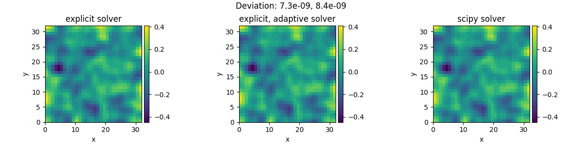
2.4.8 Solver comparison

This example shows how to set up solvers explicitly and how to extract diagnostic information.

Diagnostic information from first run:
{'controller': {'mpi_run': False, 't_start': 0, 't_end': 1.0, 'profiler': {'solver': 0.0053741849999937585, 'tracker': 3.612999999802469e-05, 'compilation': 8.759453668000006}, 'jit_count': {'make_stepper': 10, 'simulation': 0}, 'solver_start': '2025-05-24 15:38:14.440164', 'successful': True, 'stop_reason': 'Reached final time', 'solver_duration': '0:00:00.005405', 't_final': 1.0}, 'package_version': 'unknown', 'solver': {'class': 'ExplicitSolver', 'pde_class': 'DiffusionPDE', 'scheme': 'euler', 'backend': 'numba', 'dt': 0.001, 'steps': 1000, 'post_step_data': None, 'stochastic': np.False_}}

Diagnostic information from second run:
{'controller': {'mpi_run': False, 't_start': 0, 't_end': 1.0, 'profiler': {'solver': 0.08682866699999181, 'tracker': 3.581000001418033e-05, 'compilation': 2.266394313999996}, 'jit_count': {'make_stepper': 1, 'simulation': 0}, 'solver_start': '2025-05-24 15:38:16.713157', 'successful': True, 'stop_reason': 'Reached final time', 'solver_duration': '0:00:00.087096', 't_final': np.float64(1.0)}, 'package_version': 'unknown', 'solver': {'class': 'ExplicitSolver', 'pde_class': 'DiffusionPDE', 'dt_statistics': {'min': 0.001, 'max': 0.1690822072051333, 'mean': 0.08333333333333333, 'std': 0.051707546359477996, 'count': 12.0}, 'scheme': 'runge-kutta', 'backend': 'numba', 'dt': 0.001, 'dt_adaptive': True, 'steps': 12, 'stochastic': np.False_, 'post_step_data': None}}

Diagnostic information from third run:
{'controller': {'mpi_run': False, 't_start': 0, 't_end': 1.0, 'profiler': {'solver': 0.0012670910000025515, 'tracker': 3.288000000623015e-05, 'compilation': 1.9059541359999912}, 'jit_count': {'make_stepper': 1, 'simulation': 0}, 'solver_start': '2025-05-24 15:38:19.490997', 'successful': True, 'stop_reason': 'Reached final time', 'solver_duration': '0:00:00.001294', 't_final': np.float64(1.0)}, 'package_version': 'unknown', 'solver': {'class': 'ScipySolver', 'pde_class': 'DiffusionPDE', 'dt': None, 'steps': 50, 'stochastic': False, 'backend': 'numba'}}

import pde

# initialize the grid, an initial condition, and the PDE
grid = pde.UnitGrid([32, 32])
field = pde.ScalarField.random_uniform(grid, -1, 1)
eq = pde.DiffusionPDE()

# try the explicit solver
solver1 = pde.ExplicitSolver(eq)
controller1 = pde.Controller(solver1, t_range=1, tracker=None)
sol1 = controller1.run(field, dt=1e-3)
sol1.label = "explicit solver"
print("Diagnostic information from first run:")
print(controller1.diagnostics)
print()

# try an explicit solver with adaptive time steps
solver2 = pde.ExplicitSolver(eq, scheme="runge-kutta", adaptive=True)
controller2 = pde.Controller(solver2, t_range=1, tracker=None)
sol2 = controller2.run(field, dt=1e-3)
sol2.label = "explicit, adaptive solver"
print("Diagnostic information from second run:")
print(controller2.diagnostics)
print()

# try the standard scipy solver
solver3 = pde.ScipySolver(eq)
controller3 = pde.Controller(solver3, t_range=1, tracker=None)
sol3 = controller3.run(field)
sol3.label = "scipy solver"
print("Diagnostic information from third run:")
print(controller3.diagnostics)
print()

# plot both fields and give the deviation as the title
deviation12 = ((sol1 - sol2) ** 2).average
deviation13 = ((sol1 - sol3) ** 2).average
title = f"Deviation: {deviation12:.2g}, {deviation13:.2g}"
pde.FieldCollection([sol1, sol2, sol3]).plot(title=title)