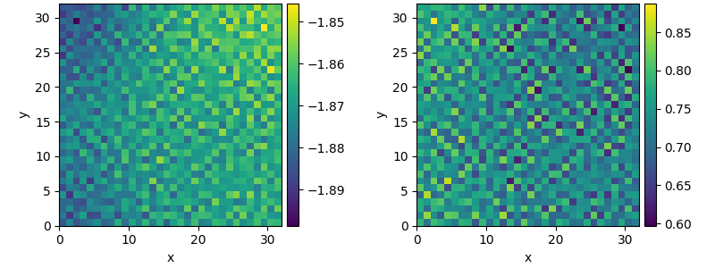
2.20. Custom Class for coupled PDEs

This example shows how to solve a set of coupled PDEs, the spatially coupled FitzHugh–Nagumo model, which is a simple model for the excitable dynamics of coupled Neurons:

\[\begin{split}\partial_t u &= \nabla^2 u + u (u - \alpha) (1 - u) + w \\ \partial_t w &= \epsilon u\end{split}\]

Here, \(\alpha\) denotes the external stimulus and \(\epsilon\) defines the recovery time scale. We implement this as a custom PDE class below.

  0%|          | 0/100.0 [00:00<?, ?it/s]
Initializing:   0%|          | 0/100.0 [00:00<?, ?it/s]
  0%|          | 0/100.0 [00:00<?, ?it/s]
  0%|          | 0.23/100.0 [00:00<01:45,  1.06s/it]
  1%|          | 0.69/100.0 [00:00<00:42,  2.36it/s]
  3%|2         | 2.77/100.0 [00:00<00:17,  5.66it/s]
  7%|7         | 7.46/100.0 [00:00<00:11,  7.94it/s]
 14%|#4        | 14.45/100.0 [00:01<00:09,  8.61it/s]
 23%|##2       | 22.58/100.0 [00:02<00:08,  8.78it/s]
 31%|###1      | 31.18/100.0 [00:03<00:07,  9.17it/s]
 41%|####      | 40.64/100.0 [00:04<00:06,  9.38it/s]
 50%|#####     | 50.42/100.0 [00:05<00:05,  9.32it/s]
 60%|#####9    | 59.84/100.0 [00:06<00:04,  9.46it/s]
 70%|######9   | 69.69/100.0 [00:07<00:03,  9.53it/s]
 80%|#######9  | 79.63/100.0 [00:08<00:02,  9.48it/s]
 89%|########9 | 89.16/100.0 [00:09<00:01,  9.54it/s]
 99%|#########8| 98.94/100.0 [00:10<00:00,  9.58it/s]
 99%|#########8| 98.94/100.0 [00:10<00:00,  9.47it/s]
100%|##########| 100.0/100.0 [00:10<00:00,  9.58it/s]
100%|##########| 100.0/100.0 [00:10<00:00,  9.58it/s]

from pde import FieldCollection, PDEBase, UnitGrid


class FitzhughNagumoPDE(PDEBase):
    """FitzHugh–Nagumo model with diffusive coupling"""

    def __init__(self, stimulus=0.5, τ=10, a=0, b=0, bc="auto_periodic_neumann"):
        super().__init__()
        self.bc = bc
        self.stimulus = stimulus
        self.τ = τ
        self.a = a
        self.b = b

    def evolution_rate(self, state, t=0):
        v, w = state  # membrane potential and recovery variable

        v_t = v.laplace(bc=self.bc) + v - v**3 / 3 - w + self.stimulus
        w_t = (v + self.a - self.b * w) / self.τ

        return FieldCollection([v_t, w_t])


grid = UnitGrid([32, 32])
state = FieldCollection.scalar_random_uniform(2, grid)

eq = FitzhughNagumoPDE()
result = eq.solve(state, t_range=100, dt=0.01)
result.plot()