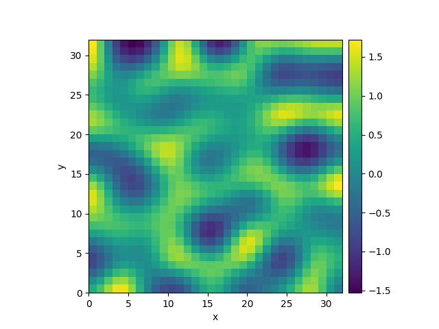
2.2.4 Kuramoto-Sivashinsky - Using PDE class

This example implements a scalar PDE using the PDE. We here consider the Kuramoto–Sivashinsky equation, which for instance describes the dynamics of flame fronts:

\[\partial_t u = -\frac12 |\nabla u|^2 - \nabla^2 u - \nabla^4 u\]

  0%|          | 0/10.0 [00:00<?, ?it/s]
Initializing:   0%|          | 0/10.0 [00:00<?, ?it/s]
  0%|          | 0/10.0 [00:11<?, ?it/s]
  0%|          | 0.01/10.0 [00:21<5:54:21, 2128.27s/it]
  0%|          | 0.02/10.0 [00:21<2:57:00, 1064.15s/it]
  2%|▏         | 0.16/10.0 [00:21<21:48, 133.02s/it]
 97%|█████████▋| 9.68/10.0 [00:21<00:00,  2.20s/it]
 97%|█████████▋| 9.68/10.0 [00:21<00:00,  2.20s/it]
100%|██████████| 10.0/10.0 [00:21<00:00,  2.13s/it]
100%|██████████| 10.0/10.0 [00:21<00:00,  2.13s/it]

from pde import PDE, ScalarField, UnitGrid

grid = UnitGrid([32, 32])  # generate grid
state = ScalarField.random_uniform(grid)  # generate initial condition

eq = PDE({"u": "-gradient_squared(u) / 2 - laplace(u + laplace(u))"})  # define the pde
result = eq.solve(state, t_range=10, dt=0.01)
result.plot()