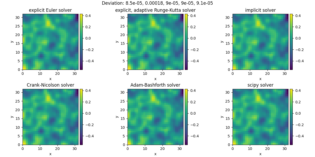
2.4.9 Solver comparison

This example shows how to set up solvers explicitly and how to extract diagnostic information.

Diagnostic information for explicit Euler solver:
{'controller': {'mpi_run': False, 't_start': 0, 't_end': 1.0, 'profiler': {'solver': 0.004776124000002824, 'tracker': 2.775000000099226e-05, 'compilation': 4.019105049000004}, 'jit_count': {'make_stepper': 10, 'simulation': 0}, 'solver_start': '2025-09-30 07:23:28.258416', 'successful': True, 'stop_reason': 'Reached final time', 'solver_duration': '0:00:00.004799', 't_final': 1.0}, 'package_version': 'unknown', 'solver': {'class': 'ExplicitSolver', 'pde_class': 'DiffusionPDE', 'scheme': 'euler', 'backend': 'numba', 'dt': 0.001, 'dt_adaptive': False, 'steps': 1000, 'post_step_data': None, 'stochastic': False}}

Diagnostic information for explicit, adaptive Runge-Kutta solver:
{'controller': {'mpi_run': False, 't_start': 0, 't_end': 1.0, 'profiler': {'solver': 0.0009463100000033364, 'tracker': 2.657999999655658e-05, 'compilation': 0.6086947390000006}, 'jit_count': {'make_stepper': 1, 'simulation': 0}, 'solver_start': '2025-09-30 07:23:28.872265', 'successful': True, 'stop_reason': 'Reached final time', 'solver_duration': '0:00:00.000968', 't_final': np.float64(1.0)}, 'package_version': 'unknown', 'solver': {'class': 'ExplicitSolver', 'pde_class': 'DiffusionPDE', 'dt_statistics': {'min': 0.001, 'max': 0.16575002695259963, 'mean': 0.08333333333333334, 'std': 0.05141575657521199, 'count': 12.0}, 'scheme': 'runge-kutta', 'backend': 'numba', 'dt': 0.001, 'dt_adaptive': True, 'steps': 12, 'stochastic': False, 'post_step_data': None}}

Diagnostic information for implicit solver:
{'controller': {'mpi_run': False, 't_start': 0, 't_end': 1.0, 'profiler': {'solver': 0.8427446879999962, 'tracker': 4.0560000002187735e-05, 'compilation': 0.6153911229999949}, 'jit_count': {'make_stepper': 1, 'simulation': 0}, 'solver_start': '2025-09-30 07:23:29.489078', 'successful': True, 'stop_reason': 'Reached final time', 'solver_duration': '0:00:00.842825', 't_final': 1.0}, 'package_version': 'unknown', 'solver': {'class': 'ImplicitSolver', 'pde_class': 'DiffusionPDE', 'function_evaluations': 0, 'scheme': 'implicit-euler', 'stochastic': False, 'backend': 'numba', 'dt': 0.001, 'dt_adaptive': False, 'steps': 1000, 'post_step_data': None}}

Diagnostic information for Crank-Nicolson solver:
{'controller': {'mpi_run': False, 't_start': 0, 't_end': 1.0, 'profiler': {'solver': 0.8647011850000013, 'tracker': 4.115999999498854e-05, 'compilation': 0.613212261000001}, 'jit_count': {'make_stepper': 1, 'simulation': 0}, 'solver_start': '2025-09-30 07:23:30.945650', 'successful': True, 'stop_reason': 'Reached final time', 'solver_duration': '0:00:00.864864', 't_final': 1.0}, 'package_version': 'unknown', 'solver': {'class': 'CrankNicolsonSolver', 'pde_class': 'DiffusionPDE', 'function_evaluations': 0, 'scheme': 'implicit-euler', 'stochastic': False, 'backend': 'numba', 'dt': 0.001, 'dt_adaptive': False, 'steps': 1000, 'post_step_data': None}}

Diagnostic information for Adam-Bashforth solver:
{'controller': {'mpi_run': False, 't_start': 0, 't_end': 1.0, 'profiler': {'solver': 0.010229988000006074, 'tracker': 2.772999999933745e-05, 'compilation': 0.6144992210000026}, 'jit_count': {'make_stepper': 1, 'simulation': 0}, 'solver_start': '2025-09-30 07:23:32.425510', 'successful': True, 'stop_reason': 'Reached final time', 'solver_duration': '0:00:00.010252', 't_final': 1.0}, 'package_version': 'unknown', 'solver': {'class': 'AdamsBashforthSolver', 'pde_class': 'DiffusionPDE', 'backend': 'numba', 'dt': 0.001, 'dt_adaptive': False, 'steps': 1000, 'post_step_data': None, 'stochastic': False}}

Diagnostic information for scipy solver:
{'controller': {'mpi_run': False, 't_start': 0, 't_end': 1.0, 'profiler': {'solver': 0.0014496109999981854, 'tracker': 2.8290000003039495e-05, 'compilation': 0.6145599230000016}, 'jit_count': {'make_stepper': 1, 'simulation': 0}, 'solver_start': '2025-09-30 07:23:33.050667', 'successful': True, 'stop_reason': 'Reached final time', 'solver_duration': '0:00:00.001472', 't_final': np.float64(1.0)}, 'package_version': 'unknown', 'solver': {'class': 'ScipySolver', 'pde_class': 'DiffusionPDE', 'dt': 0.001, 'steps': 61, 'stochastic': False, 'backend': 'numba'}}

import pde

# initialize the grid, an initial condition, and the PDE
grid = pde.UnitGrid([32, 32])
field = pde.ScalarField.random_uniform(grid, -1, 1)
eq = pde.DiffusionPDE()


def run_solver(solver, label):
    """Helper function testing the solver."""
    controller = pde.Controller(solver, t_range=1, tracker=None)
    sol = controller.run(field, dt=1e-3)
    sol.label = label + " solver"
    print(f"Diagnostic information for {sol.label}:")
    print(controller.diagnostics)
    print()
    return sol


# try different solvers
solutions = [
    run_solver(pde.ExplicitSolver(eq), "explicit Euler"),
    run_solver(
        pde.ExplicitSolver(eq, scheme="runge-kutta", adaptive=True),
        "explicit, adaptive Runge-Kutta",
    ),
    run_solver(pde.ImplicitSolver(eq), "implicit"),
    run_solver(pde.CrankNicolsonSolver(eq), "Crank-Nicolson"),
    run_solver(pde.AdamsBashforthSolver(eq), "Adam-Bashforth"),
    run_solver(pde.ScipySolver(eq), "scipy"),
]

# plot both fields and give the deviation as the title
deviations = [(solutions[0] - sol).fluctuations for sol in solutions]
title = "Deviation: " + ", ".join(f"{deviation:.2g}" for deviation in deviations[1:])
pde.FieldCollection(solutions).plot(title=title, arrangement=(2, 3))