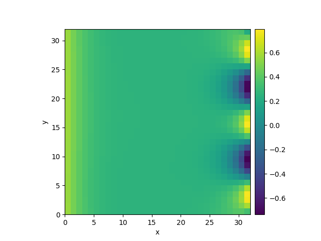
2.11. Setting boundary conditions

This example shows how different boundary conditions can be specified.

  0%|          | 0/10.0 [00:00<?, ?it/s]
Initializing:   0%|          | 0/10.0 [00:00<?, ?it/s]
  0%|          | 0/10.0 [00:08<?, ?it/s]
  0%|          | 0.005/10.0 [00:09<5:11:44, 1871.43s/it]
  0%|          | 0.01/10.0 [00:10<2:52:25, 1035.58s/it]
  0%|          | 0.015/10.0 [00:10<1:54:53, 690.41s/it]
  2%|2         | 0.23/10.0 [00:10<07:19, 45.03s/it]
  2%|2         | 0.23/10.0 [00:10<07:20, 45.09s/it]
100%|##########| 10.0/10.0 [00:10<00:00,  1.04s/it]
100%|##########| 10.0/10.0 [00:10<00:00,  1.04s/it]

from pde import DiffusionPDE, ScalarField, UnitGrid

grid = UnitGrid([32, 32], periodic=[False, True])  # generate grid
state = ScalarField.random_uniform(grid, 0.2, 0.3)  # generate initial condition

# set boundary conditions `bc` for all axes
bc_x_left = {"derivative": 0.1}
bc_x_right = {"value": "sin(y / 2)"}
bc_x = [bc_x_left, bc_x_right]
bc_y = "periodic"
eq = DiffusionPDE(bc=[bc_x, bc_y])

result = eq.solve(state, t_range=10, dt=0.005)
result.plot()