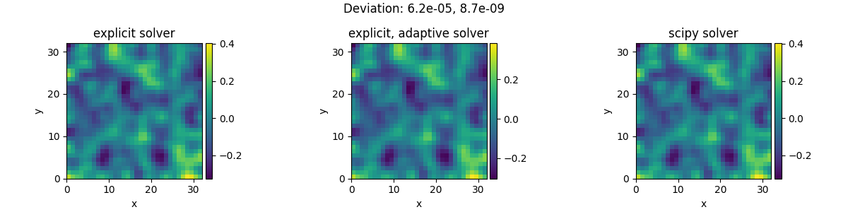
2.23. Solver comparison

This example shows how to set up solvers explicitly and how to extract diagnostic information.

Out:

Diagnostic information from first run:
{'controller': {'t_start': 0, 't_end': 1.0, 'solver_class': 'ExplicitSolver', 'solver_start': '2022-07-06 10:12:36.197643', 'profiler': {'solver': 1.4591466370000035, 'tracker': 3.57669999857535e-05}, 'successful': True, 'stop_reason': 'Reached final time', 'solver_duration': '0:00:01.459303', 't_final': 1.0}, 'package_version': '0.20.0', 'solver': {'class': 'ExplicitSolver', 'pde_class': 'DiffusionPDE', 'dt': 0.001, 'steps': 1000, 'scheme': 'euler', 'state_modifications': 0.0, 'dt_adaptive': False, 'backend': 'numba', 'stochastic': False, 'adaptive': False}, 'jit_count': {'make_stepper': 9, 'simulation': 0}}

Diagnostic information from second run:
{'controller': {'t_start': 0, 't_end': 1.0, 'solver_class': 'ExplicitSolver', 'solver_start': '2022-07-06 10:12:38.402686', 'profiler': {'solver': 2.665837649999986, 'tracker': 3.635100003407388e-05}, 'successful': True, 'stop_reason': 'Reached final time', 'solver_duration': '0:00:02.666077', 't_final': 1.08972255772386}, 'package_version': '0.20.0', 'solver': {'class': 'ExplicitSolver', 'pde_class': 'DiffusionPDE', 'dt': 0.001, 'steps': 16, 'scheme': 'runge-kutta', 'state_modifications': 0.0, 'dt_adaptive': True, 'dt_last': 0.1635705137352299, 'backend': 'numba', 'stochastic': False, 'adaptive': True}, 'jit_count': {'make_stepper': 3, 'simulation': 0}}

Diagnostic information from third run:
{'controller': {'t_start': 0, 't_end': 1.0, 'solver_class': 'ScipySolver', 'solver_start': '2022-07-06 10:12:41.824565', 'profiler': {'solver': 0.003875641999997015, 'tracker': 3.7002000027541726e-05}, 'successful': True, 'stop_reason': 'Reached final time', 'solver_duration': '0:00:00.003939', 't_final': 1.0}, 'package_version': '0.20.0', 'solver': {'class': 'ScipySolver', 'pde_class': 'DiffusionPDE', 'dt': None, 'steps': 50, 'stochastic': False, 'backend': 'numba'}, 'jit_count': {'make_stepper': 1, 'simulation': 0}}

import pde

# initialize the grid, an initial condition, and the PDE
grid = pde.UnitGrid([32, 32])
field = pde.ScalarField.random_uniform(grid, -1, 1)
eq = pde.DiffusionPDE()

# try the explicit solver
solver1 = pde.ExplicitSolver(eq)
controller1 = pde.Controller(solver1, t_range=1, tracker=None)
sol1 = controller1.run(field, dt=1e-3)
sol1.label = "explicit solver"
print("Diagnostic information from first run:")
print(controller1.diagnostics)
print()

# try an explicit solver with adaptive time steps
solver2 = pde.ExplicitSolver(eq, scheme="runge-kutta", adaptive=True)
controller2 = pde.Controller(solver2, t_range=1, tracker=None)
sol2 = controller2.run(field, dt=1e-3)
sol2.label = "explicit, adaptive solver"
print("Diagnostic information from second run:")
print(controller2.diagnostics)
print()

# try the standard scipy solver
solver3 = pde.ScipySolver(eq)
controller3 = pde.Controller(solver3, t_range=1, tracker=None)
sol3 = controller3.run(field)
sol3.label = "scipy solver"
print("Diagnostic information from third run:")
print(controller3.diagnostics)
print()

# plot both fields and give the deviation as the title
title = f"Deviation: {((sol1 - sol2)**2).average:.2g}, {((sol1 - sol3)**2).average:.2g}"
pde.FieldCollection([sol1, sol2, sol3]).plot(title=title)