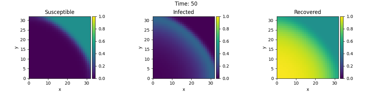
2.25 Custom PDE class: SIR model

This example implements a spatially coupled SIR model with the following dynamics for the density of susceptible, infected, and recovered individuals:

\[\begin{split}\partial_t s &= D \nabla^2 s - \beta is \\ \partial_t i &= D \nabla^2 i + \beta is - \gamma i \\ \partial_t r &= D \nabla^2 r + \gamma i\end{split}\]

Here, \(D\) is the diffusivity, \(\beta\) the infection rate, and \(\gamma\) the recovery rate.

  0%|          | 0/50.0 [00:00<?, ?it/s]
Initializing:   0%|          | 0/50.0 [00:00<?, ?it/s]
  0%|          | 0/50.0 [00:00<?, ?it/s]
  0%|          | 0.02/50.0 [00:00<30:53, 37.09s/it]
  0%|          | 0.05/50.0 [00:00<12:25, 14.92s/it]
  1%|          | 0.47/50.0 [00:00<01:24,  1.70s/it]
  5%|▍         | 2.31/50.0 [00:01<00:21,  2.26it/s]
 12%|█▏        | 6.21/50.0 [00:01<00:10,  4.16it/s]
 24%|██▍       | 11.89/50.0 [00:02<00:07,  4.98it/s]
 36%|███▌      | 17.9/50.0 [00:03<00:05,  5.74it/s]
 50%|████▉     | 24.93/50.0 [00:04<00:04,  5.97it/s]
 64%|██████▎   | 31.76/50.0 [00:05<00:02,  6.10it/s]
 77%|███████▋  | 38.49/50.0 [00:06<00:01,  6.39it/s]
 92%|█████████▏| 45.93/50.0 [00:07<00:00,  6.44it/s]
 92%|█████████▏| 45.93/50.0 [00:07<00:00,  5.87it/s]
100%|██████████| 50.0/50.0 [00:07<00:00,  6.39it/s]
100%|██████████| 50.0/50.0 [00:07<00:00,  6.39it/s]

from pde import FieldCollection, PDEBase, PlotTracker, ScalarField, UnitGrid


class SIRPDE(PDEBase):
    """SIR-model with diffusive mobility"""

    def __init__(
        self, beta=0.3, gamma=0.9, diffusivity=0.1, bc="auto_periodic_neumann"
    ):
        super().__init__()
        self.beta = beta  # transmission rate
        self.gamma = gamma  # recovery rate
        self.diffusivity = diffusivity  # spatial mobility
        self.bc = bc  # boundary condition

    def get_state(self, s, i):
        """generate a suitable initial state"""
        norm = (s + i).data.max()  # maximal density
        if norm > 1:
            s /= norm
            i /= norm
        s.label = "Susceptible"
        i.label = "Infected"

        # create recovered field
        r = ScalarField(s.grid, data=1 - s - i, label="Recovered")
        return FieldCollection([s, i, r])

    def evolution_rate(self, state, t=0):
        s, i, r = state
        diff = self.diffusivity
        ds_dt = diff * s.laplace(self.bc) - self.beta * i * s
        di_dt = diff * i.laplace(self.bc) + self.beta * i * s - self.gamma * i
        dr_dt = diff * r.laplace(self.bc) + self.gamma * i
        return FieldCollection([ds_dt, di_dt, dr_dt])


eq = SIRPDE(beta=2, gamma=0.1)

# initialize state
grid = UnitGrid([32, 32])
s = ScalarField(grid, 1)
i = ScalarField(grid, 0)
i.data[0, 0] = 1
state = eq.get_state(s, i)

# simulate the pde
tracker = PlotTracker(interrupts=10, plot_args={"vmin": 0, "vmax": 1})
sol = eq.solve(state, t_range=50, dt=1e-2, tracker=["progress", tracker])