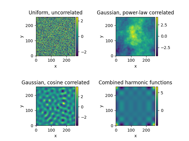
2.1.4 Random scalar fields

This example showcases several random fields

import matplotlib.pyplot as plt

from pde import ScalarField, UnitGrid

# initialize grid and plot figure
grid = UnitGrid([256, 256], periodic=True)
fig, axes = plt.subplots(nrows=2, ncols=2)

f1 = ScalarField.random_uniform(grid, -2.5, 2.5)
f1.plot(ax=axes[0, 0], title="Uniform, uncorrelated")

f2 = ScalarField.random_normal(grid, correlation="power law", exponent=-6)
f2.plot(ax=axes[0, 1], title="Gaussian, power-law correlated")

f3 = ScalarField.random_normal(grid, correlation="cosine", length_scale=30)
f3.plot(ax=axes[1, 0], title="Gaussian, cosine correlated")

f4 = ScalarField.random_harmonic(grid, modes=4)
f4.plot(ax=axes[1, 1], title="Combined harmonic functions")

plt.subplots_adjust(hspace=0.8)
plt.show()