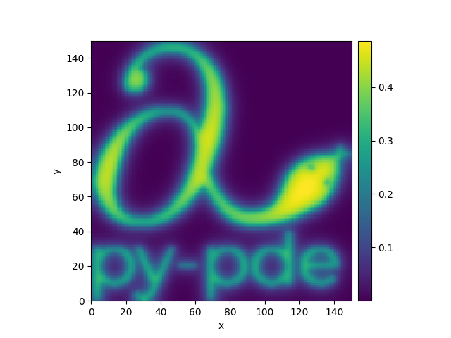
2.4.3 Heterogeneous PDE

This example loads an example image and uses it as the source field for a simple reaction-diffusion equation.

  0%|          | 0/100.0 [00:00<?, ?it/s]
Initializing:   0%|          | 0/100.0 [00:00<?, ?it/s]
  0%|          | 0/100.0 [00:22<?, ?it/s]
  0%|          | 0.00316/100.0 [00:22<195:38:28, 7043.30s/it]
  0%|          | 0.12846/100.0 [00:22<4:48:24, 173.27s/it]
  4%|▍         | 3.94661/100.0 [00:22<09:01,  5.64s/it]
 62%|██████▏   | 61.84503/100.0 [00:22<00:13,  2.78it/s]
 62%|██████▏   | 61.84503/100.0 [00:22<00:13,  2.77it/s]
100%|██████████| 100.0/100.0 [00:22<00:00,  4.49it/s]
100%|██████████| 100.0/100.0 [00:22<00:00,  4.49it/s]

import inspect
from pathlib import Path

from pde import PDE, ScalarField

# load a field relative to the current file
package_path = Path(inspect.getfile(lambda: None)).parents[2]
img_path = package_path / "docs" / "source" / "_images" / "logo_small.png"

background = ScalarField.from_image(img_path)  # create source field from image
state = ScalarField(background.grid)  # generate initial condition

# define the pde
eq = PDE({"c": "laplace(c) + 0.2 * source - 0.1 * c"}, consts={"source": background})
result = eq.solve(state, t_range=100, adaptive=True)
result.plot()