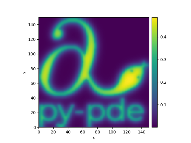
2.4.3 Heterogeneous PDE

This example loads an example image and uses it as the source field for a simple reaction-diffusion equation.

  0%|          | 0/100.0 [00:00<?, ?it/s]
Initializing:   0%|          | 0/100.0 [00:00<?, ?it/s]
  0%|          | 0/100.0 [00:07<?, ?it/s]
  0%|          | 0.00367/100.0 [00:20<151:25:46, 5451.66s/it]
  0%|          | 0.00559/100.0 [00:24<123:12:19, 4435.64s/it]
  0%|          | 0.00697/100.0 [00:24<98:48:45, 3557.50s/it]
  0%|          | 0.0726/100.0 [00:24<9:28:50, 341.55s/it]
  2%|▏         | 2.40001/100.0 [00:24<16:48, 10.33s/it]
 43%|████▎     | 42.5193/100.0 [00:24<00:33,  1.71it/s]
 43%|████▎     | 42.5193/100.0 [00:24<00:33,  1.71it/s]
100%|██████████| 100.0/100.0 [00:24<00:00,  4.03it/s]
100%|██████████| 100.0/100.0 [00:24<00:00,  4.03it/s]

import inspect
from pathlib import Path

from pde import PDE, ScalarField

# load a field relative to the current file
package_path = Path(inspect.getfile(lambda: None)).parents[2]
img_path = package_path / "docs" / "source" / "_images" / "logo_small.png"

background = ScalarField.from_image(img_path)  # create source field from image
state = ScalarField(background.grid)  # generate initial condition

# define the pde
eq = PDE({"c": "laplace(c) + 0.2 * source - 0.1 * c"}, consts={"source": background})
result = eq.solve(state, t_range=100, adaptive=True)
result.plot()