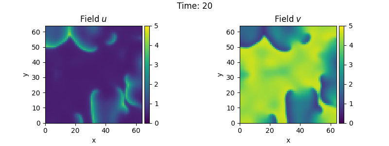
2.25. Brusselator - Using custom class

This example implements the Brusselator with spatial coupling,

\[\begin{split}\partial_t u &= D_0 \nabla^2 u + a - (1 + b) u + v u^2 \\ \partial_t v &= D_1 \nabla^2 v + b u - v u^2\end{split}\]

Here, \(D_0\) and \(D_1\) are the respective diffusivity and the parameters \(a\) and \(b\) are related to reaction rates.

Note that the PDE can also be implemented using the PDE class; see the example. However, that implementation is less flexible and might be more difficult to extend later.

import numba as nb
import numpy as np

from pde import FieldCollection, PDEBase, PlotTracker, ScalarField, UnitGrid


class BrusselatorPDE(PDEBase):
    """Brusselator with diffusive mobility"""

    def __init__(self, a=1, b=3, diffusivity=[1, 0.1], bc="auto_periodic_neumann"):
        super().__init__()
        self.a = a
        self.b = b
        self.diffusivity = diffusivity  # spatial mobility
        self.bc = bc  # boundary condition

    def get_initial_state(self, grid):
        """prepare a useful initial state"""
        u = ScalarField(grid, self.a, label="Field $u$")
        v = self.b / self.a + 0.1 * ScalarField.random_normal(grid, label="Field $v$")
        return FieldCollection([u, v])

    def evolution_rate(self, state, t=0):
        """pure python implementation of the PDE"""
        u, v = state
        rhs = state.copy()
        d0, d1 = self.diffusivity
        rhs[0] = d0 * u.laplace(self.bc) + self.a - (self.b + 1) * u + u**2 * v
        rhs[1] = d1 * v.laplace(self.bc) + self.b * u - u**2 * v
        return rhs

    def _make_pde_rhs_numba(self, state):
        """nunmba-compiled implementation of the PDE"""
        d0, d1 = self.diffusivity
        a, b = self.a, self.b
        laplace = state.grid.make_operator("laplace", bc=self.bc)

        @nb.jit
        def pde_rhs(state_data, t):
            u = state_data[0]
            v = state_data[1]

            rate = np.empty_like(state_data)
            rate[0] = d0 * laplace(u) + a - (1 + b) * u + v * u**2
            rate[1] = d1 * laplace(v) + b * u - v * u**2
            return rate

        return pde_rhs


# initialize state
grid = UnitGrid([64, 64])
eq = BrusselatorPDE(diffusivity=[1, 0.1])
state = eq.get_initial_state(grid)

# simulate the pde
tracker = PlotTracker(interval=1, plot_args={"vmin": 0, "vmax": 5})
sol = eq.solve(state, t_range=20, dt=1e-3, tracker=tracker)